Gradient descent vs coordinate descent

When it comes to function minimization, it’s time to open a book of optimization and linear algebra. I am currently working on variable selection and lasso-based solutions in genetics. What lasso does is basically minimizing the loss function and an penalty in order to set to zero some regression coefficients and select only those covariates that are really associated with the response. Pheew, the shortest summary of lasso ever!

We all know that, provided the function to be minimized is convex, a good direction to follow, in order to find a local minimum, is towards the negative gradient of the function. Now, my question is how good or bad is following the negative gradient with respect to a coordinate descent approach that loops across all dimensions and minimizes along each?

There is no better way to try this with real code and start measuring. Hence, I wrote some code that implements both gradient descent and coordinate descent.

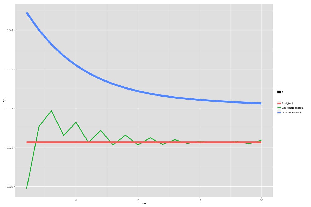
The comparison might not be completely fair because the learning rate in the gradient descent procedure is fixed at 0.1 (which in some cases might be slower indeed). But even with some tuning (maybe with some linear search) or adaptive learning rates, it’s quite common to see that coordinate descent overcomes its brother gradient descent many times.

This occurs much more often when the number of covariates becomes very high, as in many computational biology problems. In the figure below, I plot the analytical solution in red, the gradient descent minimisation in blue and the coordinate descent in green, across a number of iterations.

A small explanation is probably necessary to read the function that performs coordinate descent. For a more mathematical explanation refer to the original post.

It’s quite common to see that coordinate descent

overcomes its brother gradient descent

Coordinate descent will update each variable in a Round Robin fashion. Despite the learning rate of the gradient descent procedure (which could indeed speed up convergence), the comparison between the two is fair at least in terms of complexity.

Coordinate descent needs to perform operations for each coordinate update. Gradient descent performs the same number of operations . The R code that performs this comparison and generates the plot above is given below

library(lassoshooting) 

# make data  rm(list = ls(all = TRUE)) # make sure previous work is clear  ls() p = 70; n = 300 x <- matrix(rnorm(n*p), nrow=n, ncol=p) # create the y-matrix of dependent variables  y <- matrix(rnorm(n), nrow=n) m <- nrow(y) 

# analytical results with matrix algebra  analytical <- solve(t(x)%*%x)%*%t(x)%*%y 

# w/o feature scaling  grad <- function(x, y, theta) {   gradient <- (1/m)* (t(x) %*% ((x %*% t(theta)) - y))  return(t(gradient)) } 

# define gradient descent update algorithm  

grad.descent <- function(x, maxit){ thetas = matrix(0,ncol=dim(x)[2], nrow=maxit) theta <- matrix(0, nrow=1, ncol=dim(x)[2]) numcoord = dim(x)[2] alpha = .1 # set learning rate  for (i in 1:maxit) { theta <- theta - alpha*grad(x, y, theta) thetas[i, ] = theta } return(thetas) } 

coord.descent <- function(x, maxit, lambda=0.1){ p = dim(x)[2] theta <- matrix(0, ncol=p, nrow=maxit) # Init parameters  for(k in 1:maxit){ for(i in 1:p) { iter = ifelse(k>1, yes=k-1, 1) theta[k,i] = t(x[,i])%*% (y - x[,-i]%*%theta[iter,-i])/ (t(x[,i])%*%x[,i]) theta[k,i] = softthresh(theta[k,i], lambda) } } return(theta) } 

#compute  maxiter = 20 

out_gd = grad.descent(x, maxiter) out_cd = coord.descent(x, maxiter, lambda=0) 

#prepare results and plot  library(ggplot2) out1 = data.frame(iter=1:maxiter ,p2 = out_cd[,2]) out2 = data.frame(iter=1:maxiter ,p2 = out_gd[,2]) anal = data.frame(iter=1:maxiter, p2 = analytical[2,]) ggplot(out1,aes(iter,p2)) + geom_line(aes(color="Coordinate descent"), size=1.5) + geom_line(data=out2,aes(color="Gradient descent", size=1)) + labs(color="") + geom_line(data=anal, aes(color="Analytical", size=1))

Feel free to download this code (remember to cite me and send me some cookies).

Happy descent!

Originally published at worldofpiggy.com on May 31, 2014.