Essential Guide to Transformer Models in Machine Learning

Transformer models have become the defacto standard for NLP tasks. As an example, I’m sure you’ve already seen the awesome GPT3 Transformer demos and articles detailing how much time and money it took to train.

But even outside of NLP, you can also find transformers in the fields of computer vision and music generation.

This article was written by Rahul Agarwal (WalmartLabs) and has been reposted with permission

That said, for such a useful model, transformers are still very difficult to understand. It took me multiple readings of the Google research paper first introducing transformers, and a host of blog posts to really understand how transformers work.

So, in this article I’m putting the whole idea down as simply as possible. I’ll try to keep the jargon and the technicality to a minimum, but do keep in mind that this topic is complicated. I’ll also include some basic math and try to keep things light to ensure the long journey is fun.

Here’s what I’ll cover:

• The big picture
• The building blocks of transformer models
• Encoder architecture 
• Decoder architecture
• Output Head
• Prediction time

Q: Why should I understand Transformers?

In the past, the state of the art approach to language modeling problems (put simply, predicting the next word) and translations systems was the LSTM and GRU architecture (explained here) along with the attention mechanism. However, the main problem with these architectures is that they are recurrent in nature, and their runtime increases as the sequence length increases. In other words, these architectures take a sentence and process each word in a sequential way, so as the sentence length increases, so does the whole runtime.

The transformer architecture, first explained in the paper “Attention is All You Need”, lets go of this recurrence and instead relies entirely on an attention mechanism to draw global dependencies between input and output.

Below is a picture of the full transformer as taken from the paper. It’s quite intimidating, so let’s go through each individual piece to break it down and demystify it.

Source: https://arxiv.org/pdf/1706.03762.pdf

The Big Picture

Q: So what does a transformer model do, exactly?

A transformer model can perform almost any NLP task. We can use it for language modeling, translation, or classification, and it does these tasks quickly by removing the sequential nature of the problem. In a machine translation application, the transformer converts one language to another. For a classification problem, it provides the class probability using an appropriate output layer.

Everything depends on the final output layer for the network, but the basic structure of the transformer remains quite similar for any task. For this particular post, let’s take a closer look at the machine translation example.

From a distance, the below image shows how the transformer looks for translation. It takes as input an English sentence, and returns a German sentence.

The transformer for translation

The Building Blocks of Transformer Models

Q: That’s so basic. Can you expand on the idea?

Okay, but you asked for it. Let’s go a little deeper and look at what a transformer is composed of.

A transformer is essentially a stack of encoder and decoder layers. The role of an encoder layer is to encode our English sentence into numerical form using the attention mechanism. The decoder, on the other hand, aims to use the encoded information from the encoder layers to give us the German translation.

In the figure below, the transformer is given an English sentence as input, which gets encoded using 6 encoder layers. The output from the final encoder layer then goes to each decoder layer to translate the English into German.

Data flow in a transformer model

1. Encoder Architecture

Q: Okay, but how does an encoder stack encode an English sentence exactly?

Patience, I’ll get to that soon. As I said above, the encoder stack contains six encoder layers on top of each other. This is the same as in the paper, but keep in mind that later versions of transformers use even more layers. Each encoder in the stack has essentially two main layers:

A multi-head self-attention Layer, andA position-wise fully connected feed-forward network

Very basic encoder layer

Don’t worry, I’ll explain both of those in the coming sections. Right now, just remember that the encoder layer incorporates attention and a position-wise feed-forward network.

Q: So what does this layer expect its inputs to be?

This layer expects its inputs to be of the shape

SxD 

(see the figure below), where

S 

is the source sentence length (the English sentence), and

D

is the dimension of the embedding whose weights can be trained with the network.

In this post, we will be using

D

as 512 by default, while

S

will be the maximum length of the sentence in a batch. So it normally changes with batches.

Encoder: input and output shapes are the same

As for the outputs of this layer, keep in mind that the encoder layers are stacked on top of each other. Because of this, we want an output with the same dimensions as the input so it can flow easily into the next encoder. Therefore, the output is also the shape, SxD.

Q: Okay, so I understand what goes in and what comes out, but what actually happens in the encoder layer?

Let’s go through the attention layer and the feedforward layer one by one:

A) Self-attention Layer

How self-attention works

The above figure looks daunting but it’s easy to understand; just stay with me.

Deep learning is essentially a lot of matrix calculations, and in this layer we are doing a lot of intelligent matrix calculations. The self-attention layer initializes with 3 weight matrices — Query (W_q), Key (W_k), and Value (W_v). Each of these matrices has a size of (Dxd), where d is taken as 64 in the paper. We’ll train the weights for these matrices when we train the model.

In the first calculation (Calc 1 in the figure), we create matrices Q, K, and V by multiplying the input with the respective Query, Key, and Value matrix.

Until now it is trivial and shouldn’t make any sense as we are just doing some matrix multiplications, but it is at the second calculation it gets interesting and we get to understand why we did those exact multiplications. So, let’s try to understand the output of the softmax function. We start by multiplying the Q and Kᵀ matrix to get a matrix of size (SxS) and divide it by the scalar √d. We then take a softmax to make the rows sum to one.

Intuitively, we can think of the resultant SxS matrix as the contribution of each word in another word. For example, it might look like this:

Softmax (QxKt/sqrt(d))

As you can see the diagonal entries are big. This is because the word contribution to itself is high. That is reasonable. But we can see in the above figure that the word “quick” devolves into “quick” and “fox” and the word “brown” also devolves into “brown” and “fox”. That intuitively helps us to say that both the words — “quick” and “brown” each refers to the “fox”.

Once we have this SxS matrix with contributions we multiply this matrix by the Value matrix (Sxd) of the sentence and it gives us back a matrix of shape Sxd (4×64). So what the operation actually does is replace the embedding vector of a word like “quick” with say .75 x (quick embedding) and .2x (fox embedding), so the resultant output for the word “quick” has attention embedded in itself.

Note that the output of this layer has the dimension (Sxd) and before we get done with the whole encoder we need to change it back to D=512 as we need the output of this encoder as the input of another encoder.

Q: You called this layer the multi-head self-attention layer. What is the multi-head?

Okay, let’s get to that now.

It’s called a multi-head because we use many such self-attention layers in parallel. That is, we have many self-attention layers stacked on top of each other. The number of attention layers, h, is kept as 8 in the paper. So the input X goes through many self-attention layers in parallel, each of which gives a z matrix of shape (Sxd) = 4×64. We concatenate these 8(h) matrices and again apply a final output linear layer, Wo, of size DxD.

What size do we get? For the concatenate operation we get a size of SxD(4x(64×8) = 4×512). And multiplying this output by Wo, we get the final output Z with the shape of SxD(4×512) as desired.

Also, note the relation between h,d, and D i.e. h x d = D

The full multi-headed self-attention layer

Here we finally get the output Z of shape 4×512 as intended. But before it goes into another encoder we pass it through a Feed-Forward Network.

B) Position-wise feed-forward network

Once we understand the multi-headed attention layer, the feed-forward network is actually pretty easy to understand. It’s just a combination of various linear and dropout layers on the output Z. Consequently, we’re once again looking at a lot of Matrix multiplication.

Each word goes into the feed-forward network

The feed-forward network applies itself to each position in the output Z in parallel (each position can be thought of as a word), hence the name position-wise feed-forward network. The feed-forward network also shares weights, so the length of the source sentence doesn’t matter. If it didn’t share weights, we would have to initialize a lot of such networks based on max source sentence length, and that is not feasible.

It is actually just a linear layer that gets applied to each position (or word)

With this, we’re closing in on a basic understanding of the encoder part of transformer models.

Q: In the paper, the encoder stack has something called “positional encoding” and “Add & Norm”. What are those?

Here’s the transformer model again so you don’t have to scroll back to find it.

Glad you asked. These two concepts are pretty essential to this particular architecture, so let’s discuss these steps before moving to the decoder stack.

C. Positional Encodings

Since, our model contains no recurrence and no convolution, in order for the model to make use of the order of the sequence, we must inject some information about the relative or absolute position of the tokens in the sequence. To this end, we add “positional encodings” to the input embeddings at the bottoms of both the encoder and decoder stacks (as we will see later). The positional encodings need to have the same dimension, D, as the embeddings have so that the two can be summed.

Add a static positional pattern to X

In the paper, the authors used sine and cosine functions to create positional embeddings for the different positions.

This particular mathematical equation actually generates a 2D matrix which is added to the embedding vector that goes into the first encoder step.

Put simply, it’s just a constant matrix that we add to the sentence so that the network can get the position of the word.

Positional encoding matrix for the first 300 and 3000 positions

Above is the heatmap of the position encoding matrix that we will add to the input given to the first encoder. I’m showing the heatmap for the first 300 positions (left) and the first 3000 positions (right). We can see that there is a distinct pattern provided to our Transformer to understand the position of each word. And since we are using a function comprised of sin and cos, we can also embed positional embeddings for very high positions pretty well, as seen in the second picture.

Interesting Fact: The authors also let the transformer model learn these encodings and didn’t see any difference in performance. So, they went with the above idea as it doesn’t depend on sentence length and would be fine even if the test sentence is bigger than training samples.

D. Add and Normalize

There’s one thing I didn’t mention for the sake of simplicity when explaining the encoder: the encoder architecture (and the decoder architecture) also has skip level residual connections (something akin to resnet50). So the exact encoder architecture in the paper looks like below. Simply put, it helps traverse information for a much greater length in a Deep Neural Network. Think of this like information passing in an organization, where you have access to your manager as well as to your manager’s manager.

The skip level connections help information flow in the network

2. Decoder Architecture

Q: Okay, so now I know that an encoder takes an input sentence and encodes its information in a matrix of size SxD(4×512). How does it help the decoder decode that to German?

Before understanding how the decoder does that, let’s look at the decoder stack.

The decoder stack contains 6 decoder layers in a stack (as given in the paper again) and each decoder in the stack is comprised of the following three layers:

• Masked multi-head self-attention Layer
• Multi-head self-attention Layer, and
• A position-wise fully connected feed-forward network

It also has the same positional encoding as well as the skip level connection. We already know how the multi-head attention and feed-forward network layers work, so let’s get straight to how the decoder differs in comparison to the encoder.

The decoder architecture

Q: Wait, is that the output we need flowing into the decoder as input? Why?

Another good question. I even wondered that myself, and I hope it will be clearer by the time you reach the end of this post.

To put it into perspective, in this case we can think of a transformer as a conditional language model that predicts the next word given an input word and an English sentence on which to condition upon or base its prediction on.

So, how would you train such a model? First you give the start token

<s>

, and the model predicts the first word conditioned on the English sentence. You then change the weights based on if the prediction is right or wrong, and give the start token and the first word (

<s>

der). The model predicts the second word, you change weights again, and so on. This process is inherently sequential as you can see.

The transformer decoder learns just like this, but the beauty is that it doesn’t do so in a sequential manner. Instead, it uses masking to do this calculation and thus takes the whole output sentence (although shifted right by adding an <s> token to the front) while training. Also, please note that at prediction time we won’t give the output to the network.

A) Masked Multi-Head Self Attention Layer

Q: But how does this masking work exactly?

It works like any mask; you wear it 😷. Jokes aside, this time we have a masked multi-head attention layer in our decoder. This means that we mask our shifted output (the input to the decoder) in a way that the network is never able to see the subsequent words. Otherwise it could easily copy that word while training.

So how exactly does the mask work in the masked attention layer? If you remember earlier, in the attention layer we multiplied the query (Q) and keys (K) and divided them by sqrt(d) before taking the softmax. In a masked attention layer, we add the resultant matrix before the softmax (which will be of shape (TxT)) to a masking matrix.

So in a masked layer, the function changes like so:

Q: What happens if we do that?

Let’s break it into steps. Our resultant matrix (QxK/sqrt(d)) of shape (TxT) might look something like below: (The numbers can be big as softmax is not applied yet)

“Schnelle” currently attends to both “braune” and “fuchs”

The word schnelle will now be composed of both braune and fuchs if we take the above matrix’s softmax and multiply it with the value matrix V. But we don’t want that, so we add the mask matrix to it to result in:

The mask operation applied to the matrix.

So now what happens after we do the softmax step?

“Schnelle” never attends to any word after “schnelle”.

Since e^{-inf} = 0, all positions subsequent to schnelle have been converted to 0. Now, if we multiply this matrix with the value matrix V, the vector corresponding to schnelle’s position in the Z vector passing through the decoder will not contain any information of the subsequent words braune and fuchs, just like we wanted.

That is how the transformer takes the whole shifted output sentence at once and doesn’t learn in a sequential manner. I must say, it’s pretty neat.

Q: Are you kidding? That’s awesome.

So glad you’re still with me and appreciate it, too! Now let’s go back to the decoder. The next layer in the decoder is:

B) Multi-Headed Attention Layer

As you can see in the decoder architecture, a Z vector (output of encoder) flows from the encoder to the multi-head attention layer in the decoder. This Z output from the last encoder has a special name and is often called memory. The attention layer takes as input both the encoder output and data flowing from below (shifted outputs) and uses attention. The Query vector Q is created from the data flowing in the decoder, while the Key (K) and value (V) vectors come from the encoder output.

Q: Is there a mask here?

No, there is no mask. The output coming from below is already masked and this allows every position in the decoder to attend over all the positions in the Value vector. So for every word position to be generated the decoder has access to the whole English sentence.

Here is a single attention layer (which will be part of a multi-head just like before):

Q: But won’t the shapes of Q, K, and V be different this time?

Take a look at the figure where I did the weight calculation. Also see the shapes of the resultant Z vector and how until now our weight matrices never used the target or source sentence length in any of their dimensions.

Normally, the shape cancels away in all our matrix calculations. For example, see how the S dimension cancels away in calculation 2 above? That is why while selecting the batches during training the authors of the paper talk about tight batches. In a batch, all source sentences have similar lengths. And different batches could have different source lengths.

I will now talk about the skip level connections and the feed-forward layer.

Q: Okay, so we have the skip level connections and the FF layer, and get a matrix of shape TxD after the whole decoder operation. But where is our German translation?

3. Output Head

We’re almost there now. Once, we are done with the transformer, the next thing is to add a task-specific output head on the top of the decoder output. This can be done by adding some linear layers and softmax on top to get the probability across all the words in the German vocab. We can do something like this:

As you can see, we can generate probabilities. So far we know how to do a forward pass through this transformer architecture. So let’s see how the training of such a neural net architecture works.

Training:

Until now, when we take a bird’s eye view of the structure we have something like this:

We can give an English sentence and shifted output sentence and do a forward pass to get the probabilities over the German vocabulary. So, we should be able to use a loss function like cross-entropy where the target could be the german word we want, and train the neural network using the Adam Optimizer. Just like any classification example. There’s our German.

In the paper though, the authors use slight variations of optimizers and loss. Feel free to skip the below 2 sections on KL divergence loss and the learning rate schedule if you want. We only do this to churn out more performance, and it’s not an inherent part of transformer architecture.

A) KL Divergence with Label Smoothing:

KL Divergence is the information loss that happens when the distribution P is approximated by the distribution Q. When we use the KL Divergence loss, we try to estimate the target distribution (P) using the probabilities (Q) we generate from the model. We try to minimize this information loss in the training.

Notice that in this form (without label smoothing which we’ll discuss below) this is exactly the same as cross-entropy. Given two distributions like below.

Target distribution and probability distribution for a word (token)

The KL Divergence formula just plain gives

-logq(oder)

and that is the cross-entropy loss.

In the paper, the authors used label smoothing with α = 0.1 and so the KL Divergence loss is not cross-entropy. What this means is that in the target distribution the output value is substituted by (1-α) and the remaining 0.1 is distributed across all the words. The authors say that this is so the model is not too confident.

Q: Why do we make our models less confident? That seems absurd.

Yes, it does. But you can think of it like so: when we give the target as 1 to our loss function, we have no doubt that the true label is true and others are not. But vocabulary is inherently a non-standardized target. For example, who is to say that you cannot use good in place of great? We add some confusion to our labels so our model is not too rigid.

B) A Particular Learning Rate Schedule with Adam

The authors use a learning rate scheduler to increase the learning rate until warm-up steps, and then decrease it using the function below. They used the Adam optimizer with β¹ = 0.9, β² = 0.98. Nothing too interesting here, just some learning choices.

Source: https://arxiv.org/pdf/1706.03762.pdf

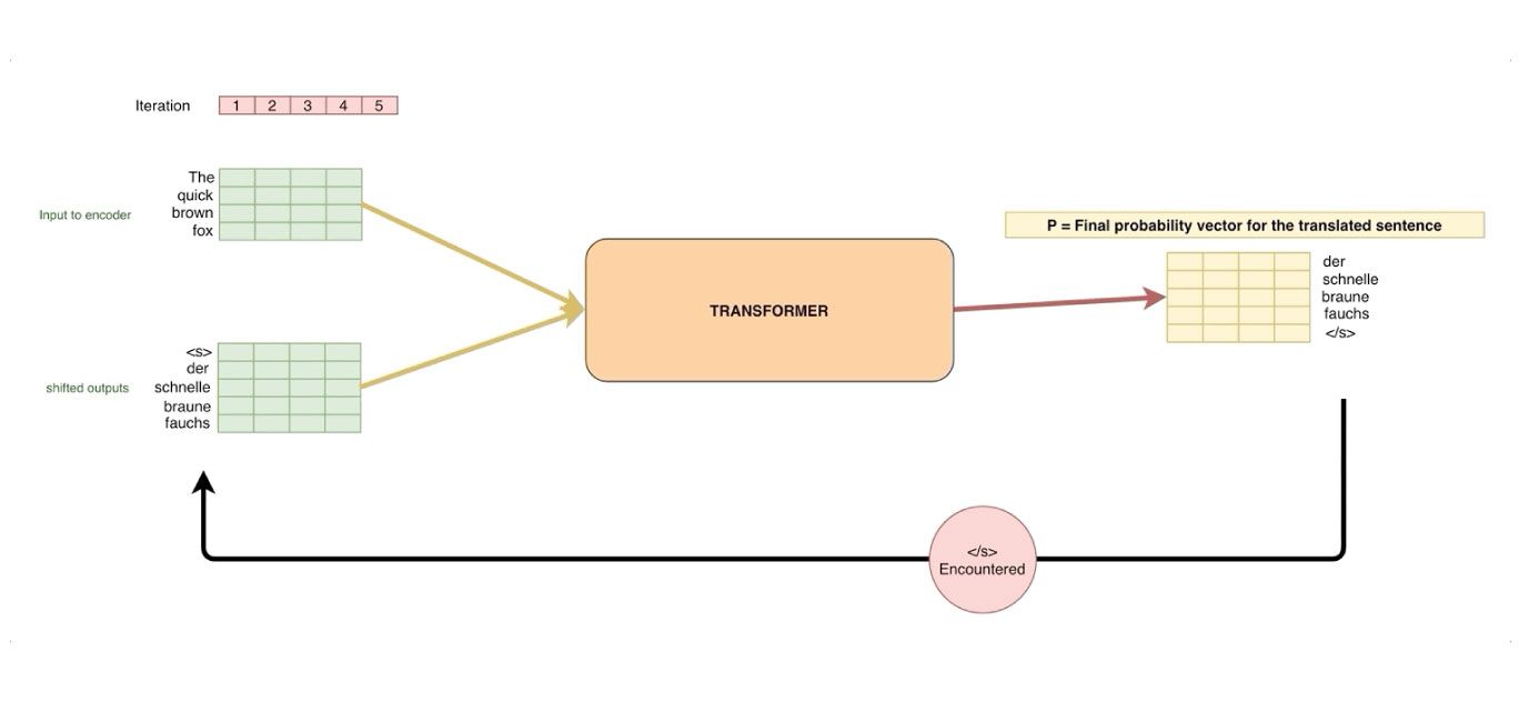
Q: I just remembered that we won’t have the shifted output at prediction time. So how do we make predictions?

What we have at this point is a generative model, so we will have to do the predictions in a generative way as we won’t know the output target vector when doing predictions. So predictions are still sequential.

Prediction Time

Predicting with a greedy search using the Transformer

This model does

piece-wise predictions. In the original paper, they use the beam search for prediction. However, a greedy search works fine for the purpose of explaining it. In the above example, I have shown how a greedy search works. It’s starts like so:

• Passing the whole English sentence as encoder input and just the start token
  

  <st> 

  as shifted output (input to the decoder) to the model and doing the forward pass.
  
• The model will predict the next word

  —der
  

• Then, we pass the whole English sentence as encoder input and add the last predicted word to the shifted output. Input to the decoder:
  

  <st>
  der 
  

  and do the forward pass.
  
• The model will predict the next word

  schnelle
  

• Passing the whole English sentence as encoder input and

  <st> der schnelle

  
  as shifted output (input to the decoder) to the model and doing the forward pass.
  
• This goes on until the model predicts the end token

  </s> 

  or we generate some maximum number of tokens (something we can define) so the translation doesn’t run for an infinite duration in the case that it breaks.

Beam Search

Q: Okay, explain the beam search to me as well.

Okay, the beam search idea is inherently very similar to the above idea. In beam search, we don’t just look at the highest probability word generated, but the top two words.

So, For example, when we gave the whole English sentence as encoder input and just the start token as shifted output, we get two best words as

i

(p=0.6) and

der

(p=0.3). We will now generate the output model for both output sequences,

<s> i

and

<s> der

and look at the probability of the next top word generated. For example, if

<s> i

gave a probability of (p=0.05) for the next word and

<s> der 

gave (p=0.5) for the next predicted word, we discard the sequence

<s> i

and go with

<s> der

instead, as the sum of probability of sentence is maximized (

<s> der next_word_to_der

p = 0.3+0.5 compared to

<s> i next_word_to__i

p = 0.6+0.05).

We then repeat this process to get the sentence with the highest probability.

Since we used the top 2 words, the beam size is 2 for this beam search. In the paper, they used beam search of size 4.

P.S. For brevity, I showed that the English sentence is passed at every step. However, in practice the output of the encoder is saved and only the shifted output passes through the decoder at each time step.

Q: Anything else you forgot?

Well, since you asked:

BPE, Weight Sharing and Checkpointing

In the paper, the authors used Byte pair encoding to create a common English-German vocabulary. They then used shared weights across both the English and German embedding and pre-softmax linear transformation as the embedding weight matrix shape would work (Vocab Length X D).

Also, the authors average the last k checkpoints to create an ensemble effect to reach the performance. This is a pretty known technique where we average the weights in the last few epochs of the model to create a new model which is sort of an ensemble.

In this post, I covered how transformer models work. If you’re interested in more technical machine learning articles, check out my other articles in the related resources section below. Also be sure to check out my podcast on the state of AI in 2020:

References

• Attention Is All You Need: The Paper that started it all.
• The Annotated Transformer: This has all the code. I’ll write a simple transformer model in my next post!
• The Illustrated Transformer: This is one of the best posts on transformers
  

This article was written by Rahul Agarwal (WalmartLabs) and has been reposted with permission.

About Rahul Agarwal

Rahul is a data scientist currently working with WalmartLabs. He enjoys working with data-intensive problems and is constantly in search of new ideas to work on. Contact him on Twitter: @MLWhiz