“Close up of modern metal sculpture of human face at Canary Wharf” by on Clem Onojeghuo Unsplash Train and evaluate a world-class deep learning model in 4 lines of code, and under 21 seconds by Stephen Rimac The following contains notes and code, compiled from a lecture given by , co-founder of . Many thanks to Jeremy and for building fast.ai and the , a high-level wrapper for . The following code is based on the fast.ai libary. For more information, watch the first lesson (of seven) in Practical For Coders, Part 1, which is publically available free of charge. If you are keen to learning deep learning, you won’t regret it! python Jeremy Howard fast.ai Rachel Thomas fast.ai library PyTorch Deep Learning Table of Contents Introduction to our first task: ‘Dogs vs Cats’ First look at cat pictures Model Analyzing results: looking at pictures 1. Introduction to our first task: Dogs vs Cats We’re going to use convolutional neural networks (CNNs) to allow our computer to see — something that is only possible thanks to deep learning. We’re going to try to create a deep learning CNN model based on data from a previous Kaggle competion called . There are available for training, and 12,500 in the test set that we have to try to label for this competition. According to the Kaggle web-site, when this competition was launched (end of 2013): Dogs vs Cats 25,000 labelled dog and cat photos “State of the art: The current literature suggests machine classifiers can score above 80% accuracy on this task”. So if we can beat 80%, then we will be at the cutting edge as of 2013! Ok, let’s going. Put these at the top of every notebook, to get automatic reloading and inline plotting: %reload_ext autoreload%autoreload 2%matplotlib inline Here we import the libraries we need: * * * * * * * from fastai.imports import from fastai.transforms import from fastai.conv_learner import from fastai.model import from fastai.dataset import from fastai.sgdr import from fastai.plots import PATH = "data/dogscats/" We set the size below to because uses 224 x 224 image sizes. More on this later: 224 resnet sz=224 Data download The dataset is available at . You can download it directly on your server by running the following line in your terminal. . You should put the data in a subdirectory of your Jupyter notebook's directory, called . http://files.fast.ai/data/dogscats.zip wget http://files.fast.ai/data/dogscats.zip data/ 2. First look at cat pictures The fast.ai library will assume that you have and directories. It also assumes that each dir will have subdirs for each class you wish to recognize (in this case, ‘cats’ and ‘dogs’). train valid Below will show the contents of ‘PATH’ folder; means run in bash. ! !ls {PATH} !ls {PATH}valid The following code shows what’s inside the validation cats folder. This is a standard way to share or provide image classification files. files = !ls {PATH}valid/cats | headfiles # Example: show first cat image in the cats folder img = plt.imread(f' ') {PATH} {files[0]} valid/cats/ # This is formatting string plt.imshow(img); I am cute Below code shows what the raw data looks like. This is called a aka a 3 x 3 matrix. Each cell shows red, green, and blue pixel values btwn 0 and 255. rank 3 tensor img.shape (198, 179, 3) Output: img[:4,:4] array([[[ 29, 20, 23],[ 31, 22, 25],[ 34, 25, 28],[ 37, 28, 31]], Output: \[\[ 60, 51, 54\], \[ 58, 49, 52\], \[ 56, 47, 50\], \[ 55, 46, 49\]\], \[\[ 93, 84, 87\], \[ 89, 80, 83\], \[ 85, 76, 79\], \[ 81, 72, 75\]\], \[\[104, 95, 98\], \[103, 94, 97\], \[102, 93, 96\], \[102, 93, 96\]\]\], dtype=uint8) 3. Model We’re going to use a model, that is, a model created by some one else to solve a different problem. Instead of building a model from scratch to solve a similar problem, we’ll use a model trained on (1.2 million images and 1000 classes) as a starting point. The model is a Convolutional Neural Network (CNN), a type of Neural Network that builds state-of-the-art models for computer vision. pre-trained ImageNet We will be using the as our pre-trained model. resnet34 is a version of the model that won the 2015 ImageNet competition. Here is more info on . resnet34 resnet models Here’s how to train and evalulate a model in 4 lines of code, and under 21 seconds. Under the syntax hood below is code/wrapper written by fast.ai. The fast.ai library is updated regularly and keeps up with cuttting-edge deep leaerning research. So fast.ai makes sure that best practices are always used. In turn, this works supper fast (e.g., 10–60 seconds depending on GPU) because it sits on top of Pytorch, which is a very flexible library written by facebook. dogs vs cats arch=resnet34 data = ImageClassifierData.from_paths(PATH, tfms=tfms_from_model(arch, sz)) learn = ConvLearner.pretrained(arch, data, precompute= ) True learn.fit(0.01, 3) Output: 100%|██████████| 360/360 [00:57<00:00, 6.24it/s]100%|██████████| 32/32 [00:05<00:00, 6.04it/s] epoch trn_loss val_loss accuracy0 0.045726 0.028603 0.9892581 0.039685 0.026488 0.9902342 0.041631 0.03259 0.990234 [0.032590486, 0.990234375] object contains the training and validation data. data reads in images and their labels given as sub-folder names: ImageClassifierData.from_paths : a root path of the data (used for storing trained models, precomputed values, etc) path : batch size. Default 64. bs : transformations (for data augmentations). e.g. output of . Default 'None' tfms tfms_from_model : a name of the folder that contains training images. Default 'train' trn_name : a name of the folder that contains validation images. Default 'valid' val_name : a name of the folder that contains test images. Default 'None' test_name : number of workers. Default '8' num_workers object contains the model. learn : ConvLearner.pretrained : arch. E.g., resnet34 f : previously defined data object data : include/exclude precomputed activations. Default 'False' precompute trains/fits the model through a given learning rate and epochs. In this instance, it is going to do 3 epochs with a 0.01 learning rate, meaning it is going to look at each image three times in total. learn.fit and are the values of the cross-entropy loss function. trn_loss val_loss How good is this model? Well, prior to this competition, the state of the art was 80% accuracy. But the competition resulted in a huge jump to accuracy, with the author of a popular deep learning library winning the competition. Extraordinarily, less than 4 years later, we can now beat that result in seconds! 99.0% Above model, can be used on any kind of pictures, as long as it is of things that people normally take photos of. However, things like pathology pictures or CT scans won’t do well using this model. There are some minor things we need to do to make those work. This will be covered in a subsequent notebook. Stay tuned! 4. Analyzing results: looking at pictures As well as looking at the overall metrics, it’s also a good idea to look at examples of some of the predictions: A few correct labels at random A few incorrect labels at random The most correct labels of each class (i.e., those with highest probability that are correct) The most incorrect labels of each class (i.e., those with highest probability that are incorrect) The most uncertain labels (i.e., those with probability closest to 0.5). We will look at all of this shortly. But first, if we ever want to know about the data, we can look inside with a few of the following methods: _# Pull the label (dependent variable)_data.val_y _# Pull the data classes_data.classes _# Pull the y log predictions_log_preds = learn.predict()log_preds.shape _# Pull first 10 predictions_log_preds[:10] _# from log probabilities to 0 or 1_preds = np.argmax(log_preds, axis=1) _# pr(dog); i.e., anti log_probs = np.exp(log_preds[:,1]) Plotting functions rand_by_mask(mask): np.random.choice(np.where(mask)[0], 4, replace= ) def return False rand_by_correct(is_correct): rand_by_mask((preds == data.val_y)==is_correct) def return plot_val_with_title(idxs, title):imgs = np.stack([data.val_ds[x][0] x idxs])title_probs = [probs[x] x idxs]print(title) plots(data.val_ds.denorm(imgs), rows=1, titles=title_probs) def for in for in return plots(ims, figsize=(12,6), rows=1, titles= ):f = plt.figure(figsize=figsize) i range(len(ims)):sp = f.add_subplot(rows, len(ims)//rows, i+1)sp.axis('Off') titles : sp.set_title(titles[i], fontsize=16)plt.imshow(ims[i]) def None for in if is not None load_img_id(ds, idx): np.array(PIL.Image.open(PATH+ds.fnames[idx])) def return plot_val_with_title(idxs, title):imgs = [load_img_id(data.val_ds,x) x idxs]title_probs = [probs[x] x idxs]print(title) plots(imgs, rows=1, titles=title_probs, figsize=(16,8)) def for in for in return most_by_mask(mask, mult):idxs = np.where(mask)[0] idxs[np.argsort(mult * probs[idxs])[:4]] def return most_by_correct(y, is_correct):mult = -1 (y==1)==is_correct 1 most_by_mask(((preds == data.val_y)==is_correct) & (data.val_y == y), mult) def if else return A few correct labels at random Anything greater than 0.5 is dog; anything less than 0.5 is cat: plot_val_with_title(rand_by_correct( ), "Correctly classified") True Ahhh A few incorrect labels at random Anything greater than 0.5 is dog; anything less than 0.5 is cat: plot_val_with_title(rand_by_correct( ), "Correctly classified") True Dogs? The most correct labels of each class (i.e., those with highest probability that are correct) plot_val_with_title(most_by_correct(0, ), "Most correct cats") True plot_val_with_title(most_by_correct(1, ), "Most correct dogs") True I like the grey ones The most incorrect labels of each class (i.e., those with highest probability that are incorrect) plot_val_with_title(most_by_correct(0, ), "Most incorrect cats") False plot_val_with_title(most_by_correct(1, ), "Most incorrect dogs") False The most uncertain labels (i.e., those with probability closest to 0.5) # probabilites are closest to 0.5 most_uncertain = np.argsort(np.abs(probs -0.5))[:4]plot_val_with_title(most_uncertain, "Most uncertain predictions") weird nb: The images above that are dimensionally wrong (e.g., the rectangular ones) are skewing the results. We take care of this using a technique called . More on that in a later post. data augmentation : if you want to make the model better, you might want to take advantage of why it is doing well and fix the things that it is doing badly. E.g., in another Jupyter notebook, try removing images that are just skewing the data, like cartoons, etc. If you figure out how to do this, let me know :) Pro tip See GitHub link below for all of above work. Thanks for reading! _Contribute to Image-classification-with-CNNs development by creating an account on GitHub._github.com Stephen-Rimac/Image-classification-with-CNNs