Handwriting Recognition: Recognizing handwritten text is a problem that can be traced back to the first automatic machines that needed to recognize individual characters in handwritten documents. Think about, for example, the ZIP codes on letters at the post office and the automation needed to recognize these five digits. Perfect recognition of these codes is necessary in order to sort mail automatically and efficiently. To address this issue in Python, the library provides a good example to better understand this technique, the issues involved, and the possibility of making predictions. scikit-learn The problem we are solving in this blog involves predicting a numeric value, and then reading and interpreting an image that uses a handwritten font. So even in this case, we will have an estimator with the task of learning through a fit() function, and once it has reached a degree of predictive capability (a model sufficiently valid), it will produce a prediction with the predict() function. Then we will discuss the training set and validation set, created this time from a series of images. The Digits Dataset The library provides numerous datasets that are useful for testing many problems of data analysis and prediction of the results. Also in this case there is a dataset of images called Digits. scikit-learn This dataset consists of 1,797 images that are 8x8 pixels in size Let's start with importing the dataset from scikit-learn: sklearn datasets   ## importing datasets sklearn
digits = datasets.load_digits()  ### loading data scikit_learn library from import from from (digits.DESCR) print ## getting information about the data The images of the handwritten digits are contained in a digits.images array. Each element of this array is an image that is represented by an 8x8 matrix of numerical values that correspond to grayscale from white, with a value of 0, to black, with the value 15. digits.images[ ] ([[ , , , , , , , ],
       [ , , , , , , , ],
       [ , , , , , , , ],
       [ , , , , , , , ],
       [ , , , , , , , ],
       [ , , , , , , , ],
       [ , , , , , , , ],
       [ , , , , , , , ]]) 0 array 0. 0. 5. 13. 9. 1. 0. 0. 0. 0. 13. 15. 10. 15. 5. 0. 0. 3. 15. 2. 0. 11. 8. 0. 0. 4. 12. 0. 0. 8. 8. 0. 0. 5. 8. 0. 0. 9. 8. 0. 0. 4. 11. 0. 1. 12. 7. 0. 0. 2. 14. 5. 10. 12. 0. 0. 0. 0. 6. 13. 10. 0. 0. 0. We can visually check the contents of this result using the library. matplotlib matplotlib.pyplot plt
%matplotlib plt.imshow(digits.images[ ], cmap=plt.cm.gray_r, interpolation= ) ## visualizing image import as inline 0 'nearest' of '0' digits.target  ## The numerical values represented by images, i.e. the targets ([ , , , ..., , , ])

digits.target.size  ## total images array 0 1 2 8 9 8 1797 The dataset is a training set consisting of 1,797 images. The Hypothesis to be tested: The Digits data set of library provides numerous data-sets that are useful for testing many problems of data analysis and prediction of the results. Some Scientist claims that it predicts the digit accurately 95% of the times. Perform data Analysis to accept or reject this Hypothesis. scikit-learn An estimator that is useful in this case is which uses the technique of Support Vector Classification (SVC).As it works with image datasets better compared to other machine learning algorithms. sklearn.svm.SVC, Support vector machine is one of the simple algorithms that every machine learning expert should have used in his/her arsenal. The Support vector machine is highly preferred by many as it produces significant accuracy with less computation power. Support Vector Machine, abbreviated as SVM can be used for both regression and classification tasks. But, it is widely used in classification objectives. What is Support Vector Machine? 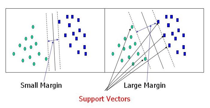The objective of the support vector machine algorithm is to find a hyperplane in N-dimensional space(N — the number of features) that distinctly classify the data points. To separate the two classes of data points, there are many possible hyperplanes that could be chosen. Our objective is to find a plane that has the maximum margin, i.e the maximum distance between data points of both classes. Maximizing the margin distance provides some reinforcement so that future data points can be classified with more confidence. Hyperplanes and Support Vectors: Hyperplanes are decision boundaries that help classify the data points. Data points falling on either side of the hyperplane can be attributed to different classes. Also, the dimension of the hyperplane depends upon the number of features. If the number of input features is 2, then the hyperplane is just a line. If the number of input features is 3, then the hyperplane becomes a two-dimensional plane. It becomes difficult to imagine when the number of features exceeds 3. Support vectors are data points that are closer to the hyperplane and influence the position and orientation of the hyperplane. Using these support vectors, we maximize the margin of the classifier. Deleting the support vectors will change the position of the hyperplane. These are the points that help us build our SVM. Large Margin Intuition: In SVM, we take the output of the linear function and if that output is greater than 1, we identify it with one class and if the output is -1, we identify is with another class. Since the threshold values are changed to 1 and -1 in SVM, we obtain this reinforcement range of values([-1,1]) which acts as margin. Cost Function and Gradient Updates: In the SVM algorithm, we are looking to maximize the margin between the data points and the hyperplane. The loss function that helps maximize the margin is hinge loss. Hinge loss function The cost is 0 if the predicted value and the actual value are of the same sign. If they are not, we then calculate the loss value. We also add a regularization parameter to the cost function. The objective of the regularization parameter is to balance the margin maximization and loss. After adding the regularization parameter, the cost functions looks as below. Loss function for SVM Now that we have the loss function, we take partial derivatives with respect to the weights to find the gradients. Using the gradients, we can update our weights. Gradients When there is no misclassification, i.e our model correctly predicts the class of our data point, we only have to update the gradient from the regularization parameter. Gradient update when no misclassification When there is a misclassification, i.e our model makes a mistake on the prediction of the class of our data point, we include the loss along with the regularization parameter to perform gradient update. Gradient Update - MIsclassification Now let's implement it using Python. sklearn import svm
svc = svm.SVC( =0.001, =100.) from gamma C once we have defined a predictive model, we must instruct it with a training set, which is a set of data in which we already know the belonging class. Given the large number of elements contained in the Digits dataset, we shall certainly obtain a very effective model, i.e., one that’s capable of recognizing with good certainty the handwritten number. This dataset contains 1,797 elements, and so you can consider the first 1,750 as a training set and will use the remaining as a validation set. We can see in detail a few of these remaining handwritten digits by using the library: matplotlib plt.subplot( )
plt.imshow(digits [ ], cmap=plt ,
interpolation= )
plt.subplot( )
plt.imshow(digits [ ], cmap=plt ,
interpolation= ) 321 .images 1750 .cm .gray_r 'nearest' 322 .images 1751 .cm .gray_r 'nearest' plt.subplot( )
plt.imshow(digits [ ], cmap=plt ,
interpolation= )
plt.subplot( )
plt.imshow(digits [ ], cmap=plt ,
interpolation= )

plt.subplot( )
plt.imshow(digits [ ], cmap=plt ,
interpolation= )
plt.subplot( )
plt.imshow(digits [ ], cmap=plt ,
interpolation= ) 323 .images 1780 .cm .gray_r 'nearest' 324 .images 1784 .cm .gray_r 'nearest' 323 .images 1795 .cm .gray_r 'nearest' 324 .images 1796 .cm .gray_r 'nearest' Training the model : Now we can train the svc estimator that we have defined earlier on the training data. svc.fit(digits.data[:1750], digits.target[:1750])  ## fitting on training SVC( =100.0, =0.001) set C gamma Now we have to test our estimator, making it interpret the validation set. svc.predict(digits.data[ : ])  ## making prediction on validation ([ , , , , , , , , , , , , , , , , , , , , , , , , , , , , , , , , , , , , , , , , , , , , ]) 1751 1796 set array 2 1 7 4 6 3 1 3 9 1 7 6 8 4 3 1 4 0 5 3 6 9 6 1 7 5 4 4 7 2 8 2 2 5 7 9 5 4 8 8 4 9 0 8 9 If we compare them with the actual digits, as follows: digits.target[ : ] ([ , , , , , , , , , , , , , , , , , , , , , , , , , , , , , , , , , , , , , , , , , , , , ]) 1751 1796 array 2 1 7 4 6 3 1 3 9 1 7 6 8 4 3 1 4 0 5 3 6 9 6 1 7 5 4 4 7 2 8 2 2 5 7 9 5 4 8 8 4 9 0 8 9 We can see that the svc estimator has learned correctly. It is able to recognize the handwritten digits, interpreting correctly all digits of the validation set. In the above case, we have got 100% accurate predictions, but this may not be the case at all times. We will be running for at least 3 cases, each case for the different range of training and validation sets. Case-1: print(svc.fit(digits.data[: ], digits.target[: ]))  ## fitting on training print(svc.predict(digits.data[ : ]))  ## making prediction on validation digits.target[ : ]

outputs:

SVC(C= , gamma= )
[ ] ([ , , , , ]) 1790 1790 set 1791 1796 set 1791 1796 100.0 0.001 4 9 0 8 9 array 4 9 0 8 9 Case_2: print(svc.fit(digits.data[: ], digits.target[: ]))  ## fitting on training print(svc.predict(digits.data[ : ]))  ## making prediction on validation digits.target[ : ]

outputs:

SVC(C= , gamma= )
[ ] ([ , , , , , , , , , , , , , , , , , , , , , , , , , , , , , , , , , , , , , , , , , , , , , , , , , , , , , , , , , , , , , , , , , , , , , , , , , , , , , , , , , , , , , , , , , , , , , , ]) 1700 1700 set 1701 1796 set 1701 1796 100.0 0.001 6 5 0 9 8 9 8 4 1 7 7 3 5 1 0 0 2 2 7 8 2 0 1 2 6 3 8 7 5 3 4 6 6 6 4 9 1 5 0 9 5 2 8 2 0 0 1 7 6 3 2 1 7 4 6 3 1 3 9 1 7 6 8 4 3 1 4 0 5 3 6 9 6 1 7 5 4 4 7 2 8 2 2 5 7 9 5 4 8 8 4 9 0 8 9 array 6 5 0 9 8 9 8 4 1 7 7 3 5 1 0 0 2 2 7 8 2 0 1 2 6 3 3 7 3 3 4 6 6 6 4 9 1 5 0 9 5 2 8 2 0 0 1 7 6 3 2 1 7 4 6 3 1 3 9 1 7 6 8 4 3 1 4 0 5 3 6 9 6 1 7 5 4 4 7 2 8 2 2 5 7 9 5 4 8 8 4 9 0 8 9 Case_3: We will take 80% of data as a training set and 20% as validation. print(svc.fit(digits.data[: ], digits.target[: ]))  ## fitting on training set

y_pred = svc.predict(digits.data[ : ])  ## making prediction on validation set

y_test = digits.target[ : ] sklearn.metrics accuracy_score, classification_report
print(accuracy_score(y_test,y_pred))
print(classification_report(y_test,y_pred))

outputs: precision    recall  f1-score   support accuracy macro avg weighted avg 1438 1438 1438 1796 1438 1796 from import 0.9636871508379888 0 1.00 0.97 0.99 35 1 0.97 1.00 0.99 36 2 1.00 1.00 1.00 34 3 1.00 0.84 0.91 37 4 0.97 0.92 0.94 37 5 0.93 1.00 0.96 37 6 1.00 1.00 1.00 37 7 1.00 1.00 1.00 36 8 0.86 0.97 0.91 32 9 0.92 0.95 0.93 37 0.96 358 0.97 0.96 0.96 358 0.97 0.96 0.96 358 In all of the above cases, we have got 96.36% accurate predictions. That is quite a remarkable performance our model has given us. I hope this blog is able to give you some insights about SVM. If you have any feedback/suggestions, feel free to reach . me I am thankful to mentors at https://internship.suvenconsultants.com for providing awesome problem statements and giving many of us a Coding Internship Experience. Thank you www.suvenconsultants.com"

Target

Visualization of Hypothesis on Meteorological data

Read My Stories

Too Long; Didn't Read

Make resilience your competitive advantage

Building Handwritten Digits Recognizer using Support Vector Machine

About Author

Comments

TOPICS

THIS ARTICLE WAS FEATURED IN

Related Stories

Untitled Story

Visualization of Hypothesis on Meteorological data

What Are Convolution Neural Networks? [ELI5]

The Noonification: Have U Been Pwned? (1/12/2023)

Goldman Sachs, Data Lineage, and Harry Potter Spells

People are still crazy about Python after twenty-five years

Visualization of Hypothesis on Meteorological data

What Are Convolution Neural Networks? [ELI5]

The Noonification: Have U Been Pwned? (1/12/2023)

Goldman Sachs, Data Lineage, and Harry Potter Spells

People are still crazy about Python after twenty-five years

Light-Mode

Classic

Newspaper

Dark-Mode

Neon Noir

Minty

HN StartUps