paint-brush
Simplifying Transformer Blocks: Additional Experiments by@autoencoder

Simplifying Transformer Blocks: Additional Experiments

by Auto Encoder: How to Ignore the Signal Noise
Auto Encoder: How to Ignore the Signal Noise HackerNoon profile picture

Auto Encoder: How to Ignore the Signal Noise

@autoencoder

Research & publications on Auto Encoders, revolutionizing data compression and...

June 19th, 2024
Read on Terminal Reader
Read this story in a terminal
Print this story
Read this story w/o Javascript
tldt arrow

Too Long; Didn't Read

Additional experiments compare linear vs cosine decay LR schedules, shaped attention vs Value-SkipInit, and sensitivity to MLP block initialization, revealing insights into their impact on model performance and training speed.
featured image - Simplifying Transformer Blocks: Additional Experiments
1x
Read by Dr. One voice-avatar

Listen to this story

Auto Encoder: How to Ignore the Signal Noise HackerNoon profile picture
Auto Encoder: How to Ignore the Signal Noise

Auto Encoder: How to Ignore the Signal Noise

@autoencoder

Research & publications on Auto Encoders, revolutionizing data compression and feature learning techniques.
Learn More
LEARN MORE ABOUT @AUTOENCODER'S
EXPERTISE AND PLACE ON THE INTERNET.

Authors:

(1) Bobby He, Department of Computer Science, ETH Zurich (Correspondence to: bobby.he@inf.ethz.ch.);

(2) Thomas Hofmann, Department of Computer Science, ETH Zurich.

Abstract and Introduction

Related Work

Preliminaries

Simplifying Transformer Blocks

Further Experimental Analysis

Discussion, Reproducibility Statement, Acknowledgements and References

A Duality Between Downweighted Residual and Restricting Updates In Linear Layers

B Block Layouts

C Additional Experiments

D Implementation Details

C ADDITIONAL EXPERIMENTS

In this section, we provide additional experiments and ablations on top of those provided in the main paper. The experiments in this section are ordered to follow the chronological order of where they are referenced (or most relevant) in the main paper.


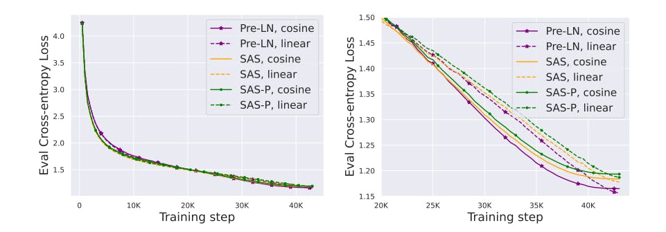
Linear vs Cosine decay LR schedule Fig. 11 compares linear and cosine decay LR schedule. We see that linear decay provides better final performance across both our models and baselines, and use linear decay throughout the rest of the paper.


Figure 11: Comparing training performance with cosine and linear decay LR schedulers on CodeParrot. The right plot is a zoomed-in version of the left. We see that linear decay consistently provides a better final performance than cosine decay, despite trailing for most of the steps towards the end of training.

Figure 11: Comparing training performance with cosine and linear decay LR schedulers on CodeParrot. The right plot is a zoomed-in version of the left. We see that linear decay consistently provides a better final performance than cosine decay, despite trailing for most of the steps towards the end of training.


Shaped Attention vs Value-SkipInit Fig. 12 explains our reasons for using Shaped Attention Eq. (5) (Noci et al., 2023) over the modified attention matrix, αI + βA(X), Eq. (4), that was introduced by He et al. (2023) in Value-SkipInit. We see that Shaped Attention gives a small but consistent gain throughout training. The experiments here follow the same training and hyperparameter setup as those in Sec. 4.


Sensitivity to MLP block gain initialisation In Sec. 4.1, we motivated downweighting the initialisation of trainable MLP block weight βFF (c.f. Eqs. (1) and (7)) in skipless architectures to replicate the implicit downweighting mechanism of Pre-LN skips. Fig. 13 shows the sensitivity of final loss to our initialisation for trainable βFF.


image

image

Figure 12: Shaped Attention (dashed lines) provides a small performance boost compared to the attention matrix of Value SkipInit (solid lines), for both SAS and SAS-P blocks. All transformers are 18-Layer autoregressive GPT models, and the dataset is CodeParrot.

Figure 12: Shaped Attention (dashed lines) provides a small performance boost compared to the attention matrix of Value SkipInit (solid lines), for both SAS and SAS-P blocks. All transformers are 18-Layer autoregressive GPT models, and the dataset is CodeParrot.


image

Figure 14: Equivalent of Fig. 3 but with tied orthogonal initialisations.

Figure 14: Equivalent of Fig. 3 but with tied orthogonal initialisations.


image


Fig. 14 is the equivalent of Fig. 3 but with LL-tied (yellow line with diamond markers) and all-tied (blue line with star markers) included. In Fig. 14, we see that matching the functional output (as in LL tied) with orthogonal initialisation provides a slight improvement to close the gap between the random orthogonal (green line) and identity (purple line) initialisations. Matching the attention sub-block outputs (as in all-tied) further improves performance, but does not fully close the gap to identity initialisation. Interestingly, it seems like orthogonally initialised values and projections do benefit from being trainable (i.e. small but non-zero βV , βP ). We leave a further exploration of these observations to future work.


image

Figs. 16 to 19 plot the corresponding trajectories, of the model in Fig. 4, for various other trainable scalar parameters we have: namely, the three shaped attention parameters 1) α on the identity (Fig. 16), 2) β on the softmax attention output (Fig. 17), 3) γ on the centring matrix (Fig. 18), as well as 4) βFF on the MLP block (Fig. 19). We see that none of these other scalar parameters converge to zero. The shaped attention parameters have error bars denoting standard deviations across (the 12) heads.


Figure 15: Corresponding plot to Fig. 4 but for a parallel block with no skips.

Figure 15: Corresponding plot to Fig. 4 but for a parallel block with no skips.


Figure 16: Trajectories for shaped attention α parameter.

Figure 16: Trajectories for shaped attention α parameter.


Figure 17: Trajectories for shaped attention β parameter

Figure 17: Trajectories for shaped attention β parameter


Figure 18: Trajectories for shaped attention γ parameter.

Figure 18: Trajectories for shaped attention γ parameter.


Figure 19: Trajectories for MLP block βFF parameter.

Figure 19: Trajectories for MLP block βFF parameter.


Identity values and projections with default Pre-LN block In Sec. 4.2 we observed that removing values and projection parameters by setting them to the identity improves the convergence speed per parameter update of transformer blocks with skipless attention sub-blocks. This raises the question of whether the same would occur in the standard block that uses attention sub-blocks skip connections i.e. the Pre-LN block. In Fig. 20 we compare the default Pre-LN block to one with values and projections set to be identity. We see that in this case identity values and projections actually slightly hurt performance in terms of loss reduction per update, in constrast to the skipless case. We also tried to downweight the attention block residual (βSA < 1 in the notation of Eq. (1)) with identity values and projections to see if the scale of the attention skip and residual was the reason for this difference, but this did not change the findings of Fig. 20. We do not have a satisfying explanation for this, but our intuition is that identity value and projections (as opposed to e.g. Gaussian/random orthogonal initialisation) with attention skip means that the two branches of the skip are no longer independent at initialisation and interfere with each other, though it is unclear that this would continue to hold during training.


image


Linearising MLP activations As stated in Sec. 4.3, we tried to use the recent idea of “linearising” activation functions in order to obtain better signal propagation (Martens et al., 2021; Zhang et al., 2022; Li et al., 2022) in deep NNs with skip connections, and recover lost training speed when the MLP skip is removed. In particular, Li et al. (2022) show for Leaky ReLU,


image


Figure 20: Pre-LN block performs worse when setting values and projections to identity, unlike in the skipless setting.

Figure 20: Pre-LN block performs worse when setting values and projections to identity, unlike in the skipless setting.


image

Figure 22: Removing MLP skips results in significant losses of training speed, even when linearising activations.

Figure 22: Removing MLP skips results in significant losses of training speed, even when linearising activations.


image

image

We see that all blocks without MLP skip train significantly slower than our SAS block (which matches the training speed of the Pre-LN block). In fact, linearising ReLU into LReLU seemed to hurt training speed rather than help it. These findings are consistent with those of previous works with AdamW optimiser (Martens et al., 2021; Zhang et al., 2022; He et al., 2023). We note that a big reason behind this is that the architectures with skipless MLP sub-blocks required an order of magnitude smaller learning rate (1e − 4 vs 1e − 3) otherwise training was unstable.


Loss vs training step In Fig. 23, we provide the equivalent plot to Fig. 5, but in terms of loss over the steps taken. Our SAS and SAS-P essentially match the Pre-LN model in terms of loss reduction per step, whilst removing normalisation slightly hurts performance.


Crammed Bert loss vs training step In Fig. 24 we plot the MLM loss in the Crammed Bert setting on the Pile dataset, as a function of the number of microbatch steps taken. Because our models have higher throughput they are able to take more steps within the 24 hour allotted time.


GLUE breakdown In Table 2, we provide a breakdown of the GLUE results in Table 1 in terms of different tasks.


Figure 23: Equivalent of Fig. 5 but with steps on the x-axis.

Figure 23: Equivalent of Fig. 5 but with steps on the x-axis.


Figure 24: MLM loss vs microbatch steps taken. Note that because the LR schedule depends on thetotal number of steps taken by a model, and is different in different models for the same number of

Figure 24: MLM loss vs microbatch steps taken. Note that because the LR schedule depends on thetotal number of steps taken by a model, and is different in different models for the same number of


This paper is available on arxiv under CC 4.0 license.


L O A D I N G
. . . comments & more!

About Author

Auto Encoder: How to Ignore the Signal Noise HackerNoon profile picture
Auto Encoder: How to Ignore the Signal Noise@autoencoder
Research & publications on Auto Encoders, revolutionizing data compression and feature learning techniques.

TOPICS

THIS ARTICLE WAS FEATURED IN...

Permanent on Arweave
Read on Terminal Reader
Read this story in a terminal
 Terminal
Read this story w/o Javascript
 Lite
Also published here