Training Neural Networks with Gorgonia

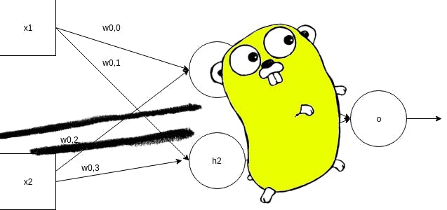
Deep learning and neural networks are very interesting subjects and Go language supports this technology using the framework Gorgonia.

Gorgonia works like similar frameworks, for example, Tensorflow, allowing the creation of graphs of operations and tensors.

There isn’t something like Keras for Gorgonia, although the project Golgi is promising.

The programming is a little low level, because we have to create the graphs containing the operations and the tensors, so there is no concept of neuron or layers, which exists in other frameworks.

In this post, I will show a very basic example of MLP - Multilayer Perceptron trying to find the weights for an approximation of the exclusive disjunction function or XOR.

Installation

First, we have to install the necessary libraries. Oh, and for starters, your Go environment has to be 1.12 or higher!

$ go version
go version go1.13.5 linux/amd64

Then, install dependency packages:

go get gorgonia.org/gorgonia

There are very useful packages, such as:

• gonum: numpy like library for Go;
• gota: pandas like library for Go;

But in this example I will use only gorgonia.

The example

I will create a two layered network, like the model:

In this model, to simplify things, it doesn’t include bias, which may make the network take a little longer to converge, but a better model It would be like this:

We have an input sequence of 4 pairs of numbers: {1,0}, {0,1}, {1,1}, {0,0}, with shape 4.2 (four lines and two columns). They are two input nodes, with four repetitions.

For this, we will have a hidden layer of 2 nodes, so we will have a weight matrix with shape 2.2 (two rows and two columns), between the inputs and the hidden layer.

And we have an exit node, so we have a weight column with shape 2.

The expected result of a XOR operation would be as follows: {1,1,0,0}.

Model Assembly and Training

The example file imports the required libraries. I will start with the interesting part, which is to create a struct to represent our neural network model:

type nn struct {
	g      *ExprGraph
	w0, w1 *Node

	pred    *Node
	predVal Value
}

This struct contains pointers to the operations graph (g), the weight layer nodes (w0 - input / hidden and w1 - hidden / output), the output node (pred) and its value (predVal).

I created a method to return the weight matrices, or learnables, what the model is expected to learn. This makes the Backpropagation part much easier:

func (m *nn) learnables() Nodes {
	return Nodes{m.w0, m.w1}
}

I also have created a factory method to instantiate the neural network:

func newNN(g *ExprGraph) *nn {
	// Create node for w/weight
	w0 := NewMatrix(g, dt, WithShape(2, 2), WithName("w0"), WithInit(GlorotN(1.0)))
	w1 := NewMatrix(g, dt, WithShape(2, 1), WithName("w1"), WithInit(GlorotN(1.0)))
	return &nn{
		g:  g,
		w0: w0,
		w1: w1}
}

Here we create two gorgonia matrices, informing their shapes and initializing with random numbers (using the Glorot algorithm).

We’re just creating nodes in the graph! Nothing will really be performed by gorgonia!

I created a method for the Forward propagation that takes the input array and passes the elements across the network:

func (m *nn) fwd(x *Node) (err error) {
	var l0, l1, l2 *Node
	var l0dot, l1dot *Node


	// Camada de input
	l0 = x

	// Multiplicação pelos pesos e sigmoid
	l0dot = Must(Mul(l0, m.w0))

	// Input para a hidden layer
	l1 = Must(Sigmoid(l0dot))

	// Multiplicação pelos pesos:
	l1dot = Must(Mul(l1, m.w1))

	// Camada de saída:
	l2 = Must(Sigmoid(l1dot))

	m.pred = l2
	Read(m.pred, &m.predVal)
	return nil

}

We multiply the entries by the weights, calculate the Sigmoid and move to the hidden layer, reaching the end.

Finally, in the main() method we instantiate our input vector and our result vector:

	// Set input x to network
	xB := []float64{1,0,0,1,1,1,0,0}
	xT := tensor.New(tensor.WithBacking(xB), tensor.WithShape(4, 2))
	x := NewMatrix(g,
		tensor.Float64,
		WithName("X"),
		WithShape(4, 2),
		WithValue(xT),
	)

	// Define validation data set
	yB := []float64{1, 1, 0, 0}
	yT := tensor.New(tensor.WithBacking(yB), tensor.WithShape(4, 1))
	y := NewMatrix(g,
		tensor.Float64,
		WithName("y"),
		WithShape(4, 1),
		WithValue(yT),
	)

Append the Forward pass in the graph:

// Run forward pass
if err := m.fwd(x); err != nil {
    log.Fatalf("%+v", err)
}

Append the loss function MSE:

// Calculate Cost w/MSE
losses := Must(Sub(y, m.pred))
square := Must(Square(losses))
cost := Must(Mean(square))

And append the gradient and Backpropagation in the graph:

// Do Gradient updates
if _, err = Grad(cost, m.learnables()...); err != nil {
    log.Fatal(err)
}

Finally, instantiate a gorgonia virtual machine and run the graph:

// Instantiate VM and Solver
vm := NewTapeMachine(g, BindDualValues(m.learnables()...))
solver := NewVanillaSolver(WithLearnRate(0.1))

for i := 0; i < 10000; i++ {
    vm.Reset()
    if err = vm.RunAll(); err != nil {
        log.Fatalf("Failed at inter  %d: %v", i, err)
    }
    solver.Step(NodesToValueGrads(m.learnables()))
    vm.Reset()
}
fmt.Println("\n\nOutput after Training: \n", m.predVal)

I repeated the training many times running the graph with vm.RunAll().

This is the training result:

Output after Training: 
 C[ 0.6267103873881292   0.6195071561964745  0.47790055401989834   0.3560452019123115]

You can create any neural network model with Gorgonia. This is just a kickstart. I didn't worry about regularization and performance, but that's a topic for another post!

Cleuton Sampaio, M.Sc.