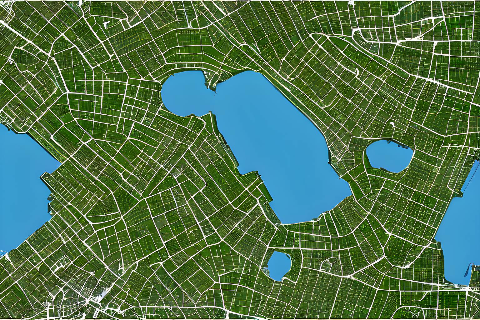
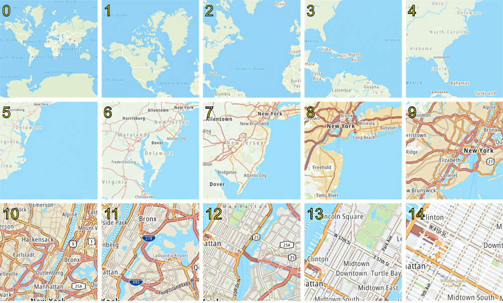
Introduction: Occasionally, you may encounter the need to perform geospatial functions within your application, such as mapping user locations or analyzing geographic data. There are numerous language-specific libraries available for these tasks, such as GDAL, Shapely, and Geopandas for Python. Alternatively, geospatial functionality can be implemented through databases; for example, you can use the PostGIS extension with a relational database like PostgreSQL, or leverage the native support for spatial data types in a distributed database like Azure CosmosDB. However, if your backend storage, such as Redis or Google Spanner, doesn't natively support spatial queries and you need to handle large-scale geospatial queries, this article is tailored for you. What Are My Options? You can always build another microservice to handle spatial data, but this option often involves the overhead of maintaining an additional application. Another approach is to use geo-indexing libraries like S2 and H3. S2, developed by Google, is based on the Hilbert curve, while H3, developed by Uber, is based on a geodesic discrete global grid system. S2 and H3 share many similarities: both divide a given region into cells and use 64-bit integers to index these cells. However, the main difference lies in the shape of the cells; S2 uses square-shaped cells, whereas H3 uses hexagon-shaped cells. For some applications, H3 might offer better performance. However, overall, either library should suffice. In this article, we will use S2, but you can perform similar functions using H3. Basic Concepts of Google S2 Library Cells: S2 divides the sphere into cells, each with a unique 64-bit identifier. Cell Levels: The hierarchy allows different levels of detail, from large regions to small precise areas. Each level represents a different resolution: Level 0: The largest cells, covering a significant portion of the Earth's surface. Higher Levels: Cells are progressively subdivided into smaller quadrants. For instance, Level 1 cells are each divided into four Level 2 cells, and so on. Resolution and Area: Higher levels correspond to finer resolutions and smaller cell areas. This hierarchy allows for precise indexing and querying at varying levels of detail. The table below shows various cell levels along with their corresponding areas. level min area max area average area units Number of cells 00 85011012.19 85011012.19 85011012.19 km2 6 01 21252753.05 21252753.05 21252753.05 km2 24 02 4919708.23 6026521.16 5313188.26 km2 96 03 1055377.48 1646455.50 1328297.07 km2 384 04 231564.06 413918.15 332074.27 km2 1536 05 53798.67 104297.91 83018.57 km2 6K 06 12948.81 26113.30 20754.64 km2 24K 07 3175.44 6529.09 5188.66 km2 98K 08 786.20 1632.45 1297.17 km2 393K 09 195.59 408.12 324.29 km2 1573K 10 48.78 102.03 81.07 km2 6M 11 12.18 25.51 20.27 km2 25M 12 3.04 6.38 5.07 km2 100M 13 0.76 1.59 1.27 km2 402M 14 0.19 0.40 0.32 km2 1610M 15 47520.30 99638.93 79172.67 m2 6B 16 11880.08 24909.73 19793.17 m2 25B 17 2970.02 6227.43 4948.29 m2 103B 18 742.50 1556.86 1237.07 m2 412B 19 185.63 389.21 309.27 m2 1649B 20 46.41 97.30 77.32 m2 7T 21 11.60 24.33 19.33 m2 26T 22 2.90 6.08 4.83 m2 105T 23 0.73 1.52 1.21 m2 422T 24 0.18 0.38 0.30 m2 1689T 25 453.19 950.23 755.05 cm2 7e15 26 113.30 237.56 188.76 cm2 27e15 27 28.32 59.39 47.19 cm2 108e15 28 7.08 14.85 11.80 cm2 432e15 29 1.77 3.71 2.95 cm2 1729e15 30 0.44 0.93 0.74 cm2 7e18 From the table provided, it's evident that you can achieve mapping precision down to 0.44 cm^2 using S2. Within each square of an S2 cell, there exists a child cell that shares the same parent, indicating a hierarchical structure. The level of the cell can be a static value (same level applied to all the cells) or can be dynamic where S2 decides what resolution works best. Calculating Nearest Neighbors Let's start with an example. Consider we are writing an application that provides proximity service-like features for the Seattle area. We want to return a list of coffee shops within the given vicinity. To perform these operations, we will divide this task into 4 sub-tasks: Loading Seattle map Visualize S2 cells on the Seattle map Store a few coffee shop locations in the database Query for nearest coffee shops Loading Seattle Map To load a Google map, we would use the gmplot library. This library requires a Google Maps API key to load. To generate the API key, follow the instructions here. import gmplot import const # plot seattle with zoom level 13 gmap = gmplot.GoogleMapPlotter(47.6061, -122.3328, 13, apikey=const.API_KEY) # Draw the map to an HTML file: gmap.draw('map.html') The above code generates a map.html file as shown below: Visualize S2 Cells on the Seattle Map Now that we have the map, let's draw some S2 cells for maps : from s2 import * import gmplot # plot seattle with zoom level 13 gmap = gmplot.GoogleMapPlotter(47.6061, -122.3328, 13, apikey=const.API_KEY) areatobeplotted = [ (47.64395531736767,-122.43597221319135), (47.51369277846956,-122.43597221319135), (47.51369277846956,-122.24156866779164), (47.64395531736767,-122.24156866779164), (47.64395531736767,-122.43597221319135) ] region_rect = S2LatLngRect( S2LatLng.FromDegrees(47.51369277846956,-122.43597221319135), S2LatLng.FromDegrees(47.64395531736767, -122.24156866779164)) coverer = S2RegionCoverer() coverer.set_min_level(8) coverer.set_max_level(15) covering = coverer.GetCovering(region_rect) geoms = 0 for cellid in covering: new_cell = S2Cell(cellid) vertices = [] for i in range(0, 4): vertex = new_cell.GetVertex(i) latlng = S2LatLng(vertex) vertices.append((latlng.lat().degrees(), latlng.lng().degrees())) gmap.polygon(*zip(*vertices), face_color='pink', edge_color='cornflowerblue', edge_width=5) geoms+=1 gmap.polygon(*zip(*areatobeplotted), face_color='red', edge_color='green', edge_width=5) print(f"Total Geometries: {geoms}") gmap.draw('/tmp/map.html') Output: Total Geometries: 273 In the code above, we first center the Google Map plotter around the Seattle area. In S2RegionCoverer, we initialize the region coverer to have dynamic levels between a minimum level of 8 and a maximum level of 15. This allows S2 to dynamically fit all cells into specific cell sizes for the best fit. The GetCovering method returns the covering for a rectangle around the Seattle area. Then, we iterate over each cell, calculating the vertices for the cells and plotting them on the map. We keep the count of cells generated to around 273. Finally, we plot the input rectangle in red. This code will plot the S2 cells on the Seattle map at /tmp/map.html, as shown below: Store a Few Coffee Shop Locations In the Database Let’s generate a database of coffee shops along with their S2 cell identifiers. You can store these cells in any database of your choice. For this tutorial, we will be using a SQLite data database. In the code sample below, we connect to the SQLite database to create a table CoffeeShops with 3 fields Id, name, and cell_id. Similar to the previous example, we use S2RegionCoverer to calculate the cells but this time, we use a fixed level for plotting points. Finally, the calculated ID is converted to a string and stored in the database. import sqlite3 from s2 import S2CellId,S2LatLng,S2RegionCoverer # Connect to SQLite database conn = sqlite3.connect('/tmp/sqlite_cells.db') cursor = conn.cursor() # Create a table to store cell IDs cursor.execute('''CREATE TABLE IF NOT EXISTS CoffeeShops ( id INTEGER PRIMARY KEY AUTOINCREMENT, name TEXT, cell_id TEXT )''') coverer = S2RegionCoverer() # Function to generate S2 cell ID for a given latitude and longitude def generate_cell_id(latitude, longitude, level=16): cell=S2CellId(S2LatLng.FromDegrees(latitude, longitude)) return str(cell.parent(level)) # Function to insert cell IDs into the database def insert_cell_ids(name,lat,lng): cell_id = generate_cell_id(lat, lng) cursor.execute("INSERT INTO CoffeeShops (name, cell_id) VALUES (?, ?)", (name, cell_id)) conn.commit() # Insert cell IDs into the database insert_cell_ids("Overcast Coffee", 47.616656277302155, -122.31156460382837) insert_cell_ids("Seattle Sunshine", 47.67366852914391, -122.29051997415843) insert_cell_ids("Sip House", 47.6682364706238, -122.31328618043693) insert_cell_ids("Victoria Coffee",47.624408595334536, -122.3117362652041) # Close connection conn.close() At this point, we have a database that stores coffee shops along with their cell IDs, determined by the selected resolution for the cell level. Query for the Nearest Coffee Shops Finally, let’s query for coffee shops in the University District area. import sqlite3 from s2 import S2RegionCoverer,S2LatLngRect, S2LatLng # Connect to SQLite database conn = sqlite3.connect('/tmp/sqlite_cells.db') cursor = conn.cursor() # Function to query database for cells intersecting with the given polygon def query_intersecting_cells(start_x,start_y,end_x,end_y): # Create S2RegionCoverer region_rect = S2LatLngRect( S2LatLng.FromDegrees(start_x,start_y), S2LatLng.FromDegrees(end_x,end_y)) coverer = S2RegionCoverer() coverer.set_min_level(8) coverer.set_max_level(15) covering = coverer.GetCovering(region_rect) # Query for intersecting cells intersecting_cells = set() for cell_id in covering: cursor.execute("SELECT name FROM CoffeeShops WHERE cell_id >= ? and cell_id<=?", (str(cell_id.range_min()),str(cell_id.range_max()),)) intersecting_cells.update(cursor.fetchall()) return intersecting_cells # Query for intersecting cells intersecting_cells = query_intersecting_cells(47.6527847,-122.3286438,47.6782181, -122.2797203) # Print intersecting cells print("Intersecting cells:") for cell_id in intersecting_cells: print(cell_id[0]) # Close connection conn.close() Output: Intersecting cells: Sip House Seattle Sunshine Below is a visual representation of the cells. To maintain brevity, the visualization code for below is not added. Since all child and parent cells share a prefix, we can query for cell ranges between min and max to get all the cells between those two values. In our example, we use the same principle to query coffee shop Conclusion: In this article, we have demonstrated how to use geo-indexing to store and query geospatial data in databases that don't support geospatial querying. This can be further extended to multiple use cases such as calculating routing between 2 points or getting nearest neighbors. Typically, for geo-indexed database querying, you would have to perform some additional post-processing on the data. Careful consideration for querying and post-processing logic is needed to ensure we don't overwhelm the node. References: Google map plotter - https://github.com/gmplot/gmplot/wiki/GoogleMapPlotter S2 developer guide - http://s2geometry.io/devguide/ Sqlite - https://docs.python.org/3/library/sqlite3.html Azure Cosmos DB geospatial - https://learn.microsoft.com/en-us/azure/cosmos-db/nosql/query/geospatial?tabs=javascript GDAL - https://gdal.org/index.html Shapley- https://shapely.readthedocs.io/en/stable/manual.html Geopandas - https://geopandas.org Posgis - https://postgis.net/ Google spanner - https://cloud.google.com/spanner?hl=en Redis - https://redis.io/ Introduction: Occasionally, you may encounter the need to perform geospatial functions within your application, such as mapping user locations or analyzing geographic data. There are numerous language-specific libraries available for these tasks, such as GDAL, Shapely, and Geopandas for Python. Alternatively, geospatial functionality can be implemented through databases; for example, you can use the PostGIS extension with a relational database like PostgreSQL, or leverage the native support for spatial data types in a distributed database like Azure CosmosDB. However, if your backend storage, such as Redis or Google Spanner, doesn't natively support spatial queries and you need to handle large-scale geospatial queries, this article is tailored for you. What Are My Options? You can always build another microservice to handle spatial data, but this option often involves the overhead of maintaining an additional application. Another approach is to use geo-indexing libraries like S2 and H3. S2, developed by Google, is based on the Hilbert curve, while H3, developed by Uber, is based on a geodesic discrete global grid system. S2 and H3 share many similarities: both divide a given region into cells and use 64-bit integers to index these cells. However, the main difference lies in the shape of the cells; S2 uses square-shaped cells, whereas H3 uses hexagon-shaped cells. For some applications, H3 might offer better performance. However, overall, either library should suffice. In this article, we will use S2, but you can perform similar functions using H3. Basic Concepts of Google S2 Library Cells: S2 divides the sphere into cells, each with a unique 64-bit identifier. Cells: S2 divides the sphere into cells, each with a unique 64-bit identifier. Cell Levels: The hierarchy allows different levels of detail, from large regions to small precise areas. Each level represents a different resolution: Level 0: The largest cells, covering a significant portion of the Earth's surface. Higher Levels: Cells are progressively subdivided into smaller quadrants. For instance, Level 1 cells are each divided into four Level 2 cells, and so on. Resolution and Area: Higher levels correspond to finer resolutions and smaller cell areas. This hierarchy allows for precise indexing and querying at varying levels of detail. Cell Levels: The hierarchy allows different levels of detail, from large regions to small precise areas. Each level represents a different resolution: Level 0: The largest cells, covering a significant portion of the Earth's surface. Higher Levels: Cells are progressively subdivided into smaller quadrants. For instance, Level 1 cells are each divided into four Level 2 cells, and so on. Resolution and Area: Higher levels correspond to finer resolutions and smaller cell areas. This hierarchy allows for precise indexing and querying at varying levels of detail. Cell Levels: The hierarchy allows different levels of detail, from large regions to small precise areas. Each level represents a different resolution: Level 0: The largest cells, covering a significant portion of the Earth's surface. Higher Levels: Cells are progressively subdivided into smaller quadrants. For instance, Level 1 cells are each divided into four Level 2 cells, and so on. Resolution and Area: Higher levels correspond to finer resolutions and smaller cell areas. This hierarchy allows for precise indexing and querying at varying levels of detail. Level 0: The largest cells, covering a significant portion of the Earth's surface. Level 0: The largest cells, covering a significant portion of the Earth's surface. Higher Levels: Cells are progressively subdivided into smaller quadrants. For instance, Level 1 cells are each divided into four Level 2 cells, and so on. Higher Levels: Cells are progressively subdivided into smaller quadrants. For instance, Level 1 cells are each divided into four Level 2 cells, and so on. Resolution and Area: Higher levels correspond to finer resolutions and smaller cell areas. This hierarchy allows for precise indexing and querying at varying levels of detail. Resolution and Area: Higher levels correspond to finer resolutions and smaller cell areas. This hierarchy allows for precise indexing and querying at varying levels of detail. The table below shows various cell levels along with their corresponding areas. level min area max area average area units Number of cells 00 85011012.19 85011012.19 85011012.19 km2 6 01 21252753.05 21252753.05 21252753.05 km2 24 02 4919708.23 6026521.16 5313188.26 km2 96 03 1055377.48 1646455.50 1328297.07 km2 384 04 231564.06 413918.15 332074.27 km2 1536 05 53798.67 104297.91 83018.57 km2 6K 06 12948.81 26113.30 20754.64 km2 24K 07 3175.44 6529.09 5188.66 km2 98K 08 786.20 1632.45 1297.17 km2 393K 09 195.59 408.12 324.29 km2 1573K 10 48.78 102.03 81.07 km2 6M 11 12.18 25.51 20.27 km2 25M 12 3.04 6.38 5.07 km2 100M 13 0.76 1.59 1.27 km2 402M 14 0.19 0.40 0.32 km2 1610M 15 47520.30 99638.93 79172.67 m2 6B 16 11880.08 24909.73 19793.17 m2 25B 17 2970.02 6227.43 4948.29 m2 103B 18 742.50 1556.86 1237.07 m2 412B 19 185.63 389.21 309.27 m2 1649B 20 46.41 97.30 77.32 m2 7T 21 11.60 24.33 19.33 m2 26T 22 2.90 6.08 4.83 m2 105T 23 0.73 1.52 1.21 m2 422T 24 0.18 0.38 0.30 m2 1689T 25 453.19 950.23 755.05 cm2 7e15 26 113.30 237.56 188.76 cm2 27e15 27 28.32 59.39 47.19 cm2 108e15 28 7.08 14.85 11.80 cm2 432e15 29 1.77 3.71 2.95 cm2 1729e15 30 0.44 0.93 0.74 cm2 7e18 level min area max area average area units Number of cells 00 85011012.19 85011012.19 85011012.19 km2 6 01 21252753.05 21252753.05 21252753.05 km2 24 02 4919708.23 6026521.16 5313188.26 km2 96 03 1055377.48 1646455.50 1328297.07 km2 384 04 231564.06 413918.15 332074.27 km2 1536 05 53798.67 104297.91 83018.57 km2 6K 06 12948.81 26113.30 20754.64 km2 24K 07 3175.44 6529.09 5188.66 km2 98K 08 786.20 1632.45 1297.17 km2 393K 09 195.59 408.12 324.29 km2 1573K 10 48.78 102.03 81.07 km2 6M 11 12.18 25.51 20.27 km2 25M 12 3.04 6.38 5.07 km2 100M 13 0.76 1.59 1.27 km2 402M 14 0.19 0.40 0.32 km2 1610M 15 47520.30 99638.93 79172.67 m2 6B 16 11880.08 24909.73 19793.17 m2 25B 17 2970.02 6227.43 4948.29 m2 103B 18 742.50 1556.86 1237.07 m2 412B 19 185.63 389.21 309.27 m2 1649B 20 46.41 97.30 77.32 m2 7T 21 11.60 24.33 19.33 m2 26T 22 2.90 6.08 4.83 m2 105T 23 0.73 1.52 1.21 m2 422T 24 0.18 0.38 0.30 m2 1689T 25 453.19 950.23 755.05 cm2 7e15 26 113.30 237.56 188.76 cm2 27e15 27 28.32 59.39 47.19 cm2 108e15 28 7.08 14.85 11.80 cm2 432e15 29 1.77 3.71 2.95 cm2 1729e15 30 0.44 0.93 0.74 cm2 7e18 level min area max area average area units Number of cells level level level min area min area min area max area max area max area average area average area average area units units units Number of cells Number of cells Number of cells 00 85011012.19 85011012.19 85011012.19 km2 6 00 00 85011012.19 85011012.19 85011012.19 85011012.19 85011012.19 85011012.19 km2 km2 6 6 01 21252753.05 21252753.05 21252753.05 km2 24 01 01 21252753.05 21252753.05 21252753.05 21252753.05 21252753.05 21252753.05 km2 km2 24 24 02 4919708.23 6026521.16 5313188.26 km2 96 02 02 4919708.23 4919708.23 6026521.16 6026521.16 5313188.26 5313188.26 km2 km2 96 96 03 1055377.48 1646455.50 1328297.07 km2 384 03 03 1055377.48 1055377.48 1646455.50 1646455.50 1328297.07 1328297.07 km2 km2 384 384 04 231564.06 413918.15 332074.27 km2 1536 04 04 231564.06 231564.06 413918.15 413918.15 332074.27 332074.27 km2 km2 1536 1536 05 53798.67 104297.91 83018.57 km2 6K 05 05 53798.67 53798.67 104297.91 104297.91 83018.57 83018.57 km2 km2 6K 6K 06 12948.81 26113.30 20754.64 km2 24K 06 06 12948.81 12948.81 26113.30 26113.30 20754.64 20754.64 km2 km2 24K 24K 07 3175.44 6529.09 5188.66 km2 98K 07 07 3175.44 3175.44 6529.09 6529.09 5188.66 5188.66 km2 km2 98K 98K 08 786.20 1632.45 1297.17 km2 393K 08 08 786.20 786.20 1632.45 1632.45 1297.17 1297.17 km2 km2 393K 393K 09 195.59 408.12 324.29 km2 1573K 09 09 195.59 195.59 408.12 408.12 324.29 324.29 km2 km2 1573K 1573K 10 48.78 102.03 81.07 km2 6M 10 10 48.78 48.78 102.03 102.03 81.07 81.07 km2 km2 6M 6M 11 12.18 25.51 20.27 km2 25M 11 11 12.18 12.18 25.51 25.51 20.27 20.27 km2 km2 25M 25M 12 3.04 6.38 5.07 km2 100M 12 12 3.04 3.04 6.38 6.38 5.07 5.07 km2 km2 100M 100M 13 0.76 1.59 1.27 km2 402M 13 13 0.76 0.76 1.59 1.59 1.27 1.27 km2 km2 402M 402M 14 0.19 0.40 0.32 km2 1610M 14 14 0.19 0.19 0.40 0.40 0.32 0.32 km2 km2 1610M 1610M 15 47520.30 99638.93 79172.67 m2 6B 15 15 47520.30 47520.30 99638.93 99638.93 79172.67 79172.67 m2 m2 6B 6B 16 11880.08 24909.73 19793.17 m2 25B 16 16 11880.08 11880.08 24909.73 24909.73 19793.17 19793.17 m2 m2 25B 25B 17 2970.02 6227.43 4948.29 m2 103B 17 17 2970.02 2970.02 6227.43 6227.43 4948.29 4948.29 m2 m2 103B 103B 18 742.50 1556.86 1237.07 m2 412B 18 18 742.50 742.50 1556.86 1556.86 1237.07 1237.07 m2 m2 412B 412B 19 185.63 389.21 309.27 m2 1649B 19 19 185.63 185.63 389.21 389.21 309.27 309.27 m2 m2 1649B 1649B 20 46.41 97.30 77.32 m2 7T 20 20 46.41 46.41 97.30 97.30 77.32 77.32 m2 m2 7T 7T 21 11.60 24.33 19.33 m2 26T 21 21 11.60 11.60 24.33 24.33 19.33 19.33 m2 m2 26T 26T 22 2.90 6.08 4.83 m2 105T 22 22 2.90 2.90 6.08 6.08 4.83 4.83 m2 m2 105T 105T 23 0.73 1.52 1.21 m2 422T 23 23 0.73 0.73 1.52 1.52 1.21 1.21 m2 m2 422T 422T 24 0.18 0.38 0.30 m2 1689T 24 24 0.18 0.18 0.38 0.38 0.30 0.30 m2 m2 1689T 1689T 25 453.19 950.23 755.05 cm2 7e15 25 25 453.19 453.19 950.23 950.23 755.05 755.05 cm2 cm2 7e15 7e15 26 113.30 237.56 188.76 cm2 27e15 26 26 113.30 113.30 237.56 237.56 188.76 188.76 cm2 cm2 27e15 27e15 27 28.32 59.39 47.19 cm2 108e15 27 27 28.32 28.32 59.39 59.39 47.19 47.19 cm2 cm2 108e15 108e15 28 7.08 14.85 11.80 cm2 432e15 28 28 7.08 7.08 14.85 14.85 11.80 11.80 cm2 cm2 432e15 432e15 29 1.77 3.71 2.95 cm2 1729e15 29 29 1.77 1.77 3.71 3.71 2.95 2.95 cm2 cm2 1729e15 1729e15 30 0.44 0.93 0.74 cm2 7e18 30 30 0.44 0.44 0.93 0.93 0.74 0.74 cm2 cm2 7e18 7e18 From the table provided, it's evident that you can achieve mapping precision down to 0.44 cm^2 using S2. Within each square of an S2 cell, there exists a child cell that shares the same parent, indicating a hierarchical structure. The level of the cell can be a static value (same level applied to all the cells) or can be dynamic where S2 decides what resolution works best. Calculating Nearest Neighbors Let's start with an example. Consider we are writing an application that provides proximity service-like features for the Seattle area. We want to return a list of coffee shops within the given vicinity. To perform these operations, we will divide this task into 4 sub-tasks: Loading Seattle map Visualize S2 cells on the Seattle map Store a few coffee shop locations in the database Query for nearest coffee shops Loading Seattle map Visualize S2 cells on the Seattle map Store a few coffee shop locations in the database Query for nearest coffee shops Loading Seattle Map To load a Google map, we would use the gmplot library. This library requires a Google Maps API key to load. To generate the API key, follow the instructions here . here import gmplot import const # plot seattle with zoom level 13 gmap = gmplot.GoogleMapPlotter(47.6061, -122.3328, 13, apikey=const.API_KEY) # Draw the map to an HTML file: gmap.draw('map.html') import gmplot import const # plot seattle with zoom level 13 gmap = gmplot.GoogleMapPlotter(47.6061, -122.3328, 13, apikey=const.API_KEY) # Draw the map to an HTML file: gmap.draw('map.html') The above code generates a map.html file as shown below: Visualize S2 Cells on the Seattle Map Now that we have the map, let's draw some S2 cells for maps : from s2 import * import gmplot # plot seattle with zoom level 13 gmap = gmplot.GoogleMapPlotter(47.6061, -122.3328, 13, apikey=const.API_KEY) areatobeplotted = [ (47.64395531736767,-122.43597221319135), (47.51369277846956,-122.43597221319135), (47.51369277846956,-122.24156866779164), (47.64395531736767,-122.24156866779164), (47.64395531736767,-122.43597221319135) ] region_rect = S2LatLngRect( S2LatLng.FromDegrees(47.51369277846956,-122.43597221319135), S2LatLng.FromDegrees(47.64395531736767, -122.24156866779164)) coverer = S2RegionCoverer() coverer.set_min_level(8) coverer.set_max_level(15) covering = coverer.GetCovering(region_rect) geoms = 0 for cellid in covering: new_cell = S2Cell(cellid) vertices = [] for i in range(0, 4): vertex = new_cell.GetVertex(i) latlng = S2LatLng(vertex) vertices.append((latlng.lat().degrees(), latlng.lng().degrees())) gmap.polygon(*zip(*vertices), face_color='pink', edge_color='cornflowerblue', edge_width=5) geoms+=1 gmap.polygon(*zip(*areatobeplotted), face_color='red', edge_color='green', edge_width=5) print(f"Total Geometries: {geoms}") gmap.draw('/tmp/map.html') from s2 import * import gmplot # plot seattle with zoom level 13 gmap = gmplot.GoogleMapPlotter(47.6061, -122.3328, 13, apikey=const.API_KEY) areatobeplotted = [ (47.64395531736767,-122.43597221319135), (47.51369277846956,-122.43597221319135), (47.51369277846956,-122.24156866779164), (47.64395531736767,-122.24156866779164), (47.64395531736767,-122.43597221319135) ] region_rect = S2LatLngRect( S2LatLng.FromDegrees(47.51369277846956,-122.43597221319135), S2LatLng.FromDegrees(47.64395531736767, -122.24156866779164)) coverer = S2RegionCoverer() coverer.set_min_level(8) coverer.set_max_level(15) covering = coverer.GetCovering(region_rect) geoms = 0 for cellid in covering: new_cell = S2Cell(cellid) vertices = [] for i in range(0, 4): vertex = new_cell.GetVertex(i) latlng = S2LatLng(vertex) vertices.append((latlng.lat().degrees(), latlng.lng().degrees())) gmap.polygon(*zip(*vertices), face_color='pink', edge_color='cornflowerblue', edge_width=5) geoms+=1 gmap.polygon(*zip(*areatobeplotted), face_color='red', edge_color='green', edge_width=5) print(f"Total Geometries: {geoms}") gmap.draw('/tmp/map.html') Output: Total Geometries: 273 Output: Total Geometries: 273 In the code above, we first center the Google Map plotter around the Seattle area. In S2RegionCoverer , we initialize the region coverer to have dynamic levels between a minimum level of 8 and a maximum level of 15. This allows S2 to dynamically fit all cells into specific cell sizes for the best fit. The GetCovering method returns the covering for a rectangle around the Seattle area. S2RegionCoverer GetCovering Then, we iterate over each cell, calculating the vertices for the cells and plotting them on the map. We keep the count of cells generated to around 273. Finally, we plot the input rectangle in red. This code will plot the S2 cells on the Seattle map at /tmp/map.html , as shown below: /tmp/map.html Store a Few Coffee Shop Locations In the Database Let’s generate a database of coffee shops along with their S2 cell identifiers. You can store these cells in any database of your choice. For this tutorial, we will be using a SQLite data database. In the code sample below, we connect to the SQLite database to create a table CoffeeShops with 3 fields Id , name , and cell_id . CoffeeShops Id name cell_id Similar to the previous example, we use S2RegionCoverer to calculate the cells but this time, we use a fixed level for plotting points. Finally, the calculated ID is converted to a string and stored in the database. S2RegionCoverer import sqlite3 from s2 import S2CellId,S2LatLng,S2RegionCoverer # Connect to SQLite database conn = sqlite3.connect('/tmp/sqlite_cells.db') cursor = conn.cursor() # Create a table to store cell IDs cursor.execute('''CREATE TABLE IF NOT EXISTS CoffeeShops ( id INTEGER PRIMARY KEY AUTOINCREMENT, name TEXT, cell_id TEXT )''') coverer = S2RegionCoverer() # Function to generate S2 cell ID for a given latitude and longitude def generate_cell_id(latitude, longitude, level=16): cell=S2CellId(S2LatLng.FromDegrees(latitude, longitude)) return str(cell.parent(level)) # Function to insert cell IDs into the database def insert_cell_ids(name,lat,lng): cell_id = generate_cell_id(lat, lng) cursor.execute("INSERT INTO CoffeeShops (name, cell_id) VALUES (?, ?)", (name, cell_id)) conn.commit() # Insert cell IDs into the database insert_cell_ids("Overcast Coffee", 47.616656277302155, -122.31156460382837) insert_cell_ids("Seattle Sunshine", 47.67366852914391, -122.29051997415843) insert_cell_ids("Sip House", 47.6682364706238, -122.31328618043693) insert_cell_ids("Victoria Coffee",47.624408595334536, -122.3117362652041) # Close connection conn.close() import sqlite3 from s2 import S2CellId,S2LatLng,S2RegionCoverer # Connect to SQLite database conn = sqlite3.connect('/tmp/sqlite_cells.db') cursor = conn.cursor() # Create a table to store cell IDs cursor.execute('''CREATE TABLE IF NOT EXISTS CoffeeShops ( id INTEGER PRIMARY KEY AUTOINCREMENT, name TEXT, cell_id TEXT )''') coverer = S2RegionCoverer() # Function to generate S2 cell ID for a given latitude and longitude def generate_cell_id(latitude, longitude, level=16): cell=S2CellId(S2LatLng.FromDegrees(latitude, longitude)) return str(cell.parent(level)) # Function to insert cell IDs into the database def insert_cell_ids(name,lat,lng): cell_id = generate_cell_id(lat, lng) cursor.execute("INSERT INTO CoffeeShops (name, cell_id) VALUES (?, ?)", (name, cell_id)) conn.commit() # Insert cell IDs into the database insert_cell_ids("Overcast Coffee", 47.616656277302155, -122.31156460382837) insert_cell_ids("Seattle Sunshine", 47.67366852914391, -122.29051997415843) insert_cell_ids("Sip House", 47.6682364706238, -122.31328618043693) insert_cell_ids("Victoria Coffee",47.624408595334536, -122.3117362652041) # Close connection conn.close() At this point, we have a database that stores coffee shops along with their cell IDs, determined by the selected resolution for the cell level. Query for the Nearest Coffee Shops Finally, let’s query for coffee shops in the University District area. import sqlite3 from s2 import S2RegionCoverer,S2LatLngRect, S2LatLng # Connect to SQLite database conn = sqlite3.connect('/tmp/sqlite_cells.db') cursor = conn.cursor() # Function to query database for cells intersecting with the given polygon def query_intersecting_cells(start_x,start_y,end_x,end_y): # Create S2RegionCoverer region_rect = S2LatLngRect( S2LatLng.FromDegrees(start_x,start_y), S2LatLng.FromDegrees(end_x,end_y)) coverer = S2RegionCoverer() coverer.set_min_level(8) coverer.set_max_level(15) covering = coverer.GetCovering(region_rect) # Query for intersecting cells intersecting_cells = set() for cell_id in covering: cursor.execute("SELECT name FROM CoffeeShops WHERE cell_id >= ? and cell_id<=?", (str(cell_id.range_min()),str(cell_id.range_max()),)) intersecting_cells.update(cursor.fetchall()) return intersecting_cells # Query for intersecting cells intersecting_cells = query_intersecting_cells(47.6527847,-122.3286438,47.6782181, -122.2797203) # Print intersecting cells print("Intersecting cells:") for cell_id in intersecting_cells: print(cell_id[0]) # Close connection conn.close() import sqlite3 from s2 import S2RegionCoverer,S2LatLngRect, S2LatLng # Connect to SQLite database conn = sqlite3.connect('/tmp/sqlite_cells.db') cursor = conn.cursor() # Function to query database for cells intersecting with the given polygon def query_intersecting_cells(start_x,start_y,end_x,end_y): # Create S2RegionCoverer region_rect = S2LatLngRect( S2LatLng.FromDegrees(start_x,start_y), S2LatLng.FromDegrees(end_x,end_y)) coverer = S2RegionCoverer() coverer.set_min_level(8) coverer.set_max_level(15) covering = coverer.GetCovering(region_rect) # Query for intersecting cells intersecting_cells = set() for cell_id in covering: cursor.execute("SELECT name FROM CoffeeShops WHERE cell_id >= ? and cell_id<=?", (str(cell_id.range_min()),str(cell_id.range_max()),)) intersecting_cells.update(cursor.fetchall()) return intersecting_cells # Query for intersecting cells intersecting_cells = query_intersecting_cells(47.6527847,-122.3286438,47.6782181, -122.2797203) # Print intersecting cells print("Intersecting cells:") for cell_id in intersecting_cells: print(cell_id[0]) # Close connection conn.close() Output: Intersecting cells: Sip House Seattle Sunshine Output: Intersecting cells: Sip House Seattle Sunshine Below is a visual representation of the cells. To maintain brevity, the visualization code for below is not added. Since all child and parent cells share a prefix, we can query for cell ranges between min and max to get all the cells between those two values. In our example, we use the same principle to query coffee shop Conclusion: In this article, we have demonstrated how to use geo-indexing to store and query geospatial data in databases that don't support geospatial querying. This can be further extended to multiple use cases such as calculating routing between 2 points or getting nearest neighbors. Typically, for geo-indexed database querying, you would have to perform some additional post-processing on the data. Careful consideration for querying and post-processing logic is needed to ensure we don't overwhelm the node. References: Google map plotter - https://github.com/gmplot/gmplot/wiki/GoogleMapPlotter S2 developer guide - http://s2geometry.io/devguide/ Sqlite - https://docs.python.org/3/library/sqlite3.html Azure Cosmos DB geospatial - https://learn.microsoft.com/en-us/azure/cosmos-db/nosql/query/geospatial?tabs=javascript GDAL - https://gdal.org/index.html Shapley- https://shapely.readthedocs.io/en/stable/manual.html Geopandas - https://geopandas.org Posgis - https://postgis.net/ Google spanner - https://cloud.google.com/spanner?hl=en Redis - https://redis.io/ Google map plotter - https://github.com/gmplot/gmplot/wiki/GoogleMapPlotter https://github.com/gmplot/gmplot/wiki/GoogleMapPlotter S2 developer guide - http://s2geometry.io/devguide/ http://s2geometry.io/devguide/ Sqlite - https://docs.python.org/3/library/sqlite3.html https://docs.python.org/3/library/sqlite3.html Azure Cosmos DB geospatial - https://learn.microsoft.com/en-us/azure/cosmos-db/nosql/query/geospatial?tabs=javascript https://learn.microsoft.com/en-us/azure/cosmos-db/nosql/query/geospatial?tabs=javascript GDAL - https://gdal.org/index.html https://gdal.org/index.html Shapley- https://shapely.readthedocs.io/en/stable/manual.html https://shapely.readthedocs.io/en/stable/manual.html Geopandas - https://geopandas.org https://geopandas.org Posgis - https://postgis.net/ https://postgis.net/ Google spanner - https://cloud.google.com/spanner?hl=en https://cloud.google.com/spanner?hl=en Redis - https://redis.io/ https://redis.io/