The study of models is a common entry point into the field of Machine Learning. Discriminative models learn a distribution that defines how one feature of a dataset depends on the others. This distribution can then be used to between data points by, for example, partitioning a dataset into classes. discriminative discriminate In addition to discriminative models, there also exist models. Rather than learn a distribution that defines features of a dataset depend on each other, generative models learn the distribution that the features themselves. This distribution can then be used to generate data that is similar to the training data. , a class of Deep Learning architectures, are one example of generative models. generative how generates new Variational Autoencoders were invented to accomplish the goal of data generation and, since their in 2013, have received great attention due to both their impressive results and underlying simplicity. Below, you will see two images of human faces. These images are not of real people - they were generated using , a DeepMind Variational Autoencoder (VAE) model. Variational Autoencoders introduction VQ-VAE 2 In this tutorial, we’ll explore how , ordinary Autoencoders, to address the challenge of data generation, and then to understand and visualize how a VAE learns. Let’s get started! Variational Autoencoders simply but powerfully extend their predecessors build and train a Variational Autoencoder with Keras If you want to jump straight to the code, you can do so . here Introduction Generating convincing data that mimics the distribution of a training set is a difficult task, one which harbors several peculiarities that make it a uniquely challenging problem. The task is unsupervised, and it necessitates that we consider the data as . That is, rather than performing operations on the data points as points to accomplish some goal that is valuable , such as clustering with K-Means, we need to determine the underlying structure of the data sufficiently enough that we can exploit it to generate convincing forgeries. Given one-million pictures of human faces, how are we to train a model that can automatically output realistic images of human faces? representative of a distribution in their own right in its own right Recall that (AEs) are a method of bottlenecking the learning of an identity map in order to find a lower-dimensional representation of a dataset, something that is useful for both dimensionality reduction and data compression. While Autoencoders are a powerful tool for these purposes, their learning objective is not designed to make them useful for generating data that is convincingly similar to a training set. Autoencoders extend the core concept of Autoencoders by placing constraints on the identity map is learned. These constraints result in VAEs characterizing the lower-dimensional space, called the , well enough that they are . VAEs characterize the latent space as a seen in the training data, rather than as a simple embedding space for data as AEs do. Variational Autoencoders how latent space useful for data generation landscape of salient features In the following sections, we will first explore how ordinary Autoencoders work, and then examine how they differ from Variational Autoencoders. We will gain an intuition for why these differences result in VAEs being well-suited for data-generation, and finally of clothing using the MNIST Fashion dataset! Let's begin by reminding ourselves what an Autoencoder is. put our knowledge to practical use by training a Variational Autoencoder to generate images ordinary What is an Autoencoder? In a wide range of data-adjacent fields, it is often beneficial to learn compressed representations of the data you are working with. You might use these lower-dimensional representations to make other Machine Learning tasks more computationally efficient, or to make data storage more space-efficient. While knowing a compressed representation of a dataset is clearly beneficial, how might we a mapping that accomplishes this compression? discover Autoencoders are a class of Neural Network architectures that learn an , which maps an input to a compressed latent space representation, and a , which maps from the latent space back into the original space. Ideally, these functions are pure inverses of each other - passing data through the encoder and then passing the result through the decoder perfectly reconstructs the original data in what is called compression. encoding function decoding function lossless A very convenient fact about Autoencoders is that, given that they are Neural Networks, they can take advantage of specialized network architectures. While there are dimensionality reduction methods that have superseded Autoencoders in terms of popularity, such as PCA and Random Projections, Autoencoders are still useful for tasks such as image compression, where ConvNets can capture local relationships in the data in a way that PCA cannot. We can use convolutional layers to map, for example, MNIST handwritten digits to a compressed form. How does the Autoencoder actually perform this compression? The convolutional layers in the network of each digit, such as the fact that an 8 is closed and has two loops, and a 9 is open and has a single loop. A fully connected network then maps these features to a lower dimensional latent space, placing it in this space according to which features are present, and to what degree, in the image. If we are already mapping images to a representative feature space, can we not use this space for image ? extract the salient features generation Can Autoencoders Be Used for Data Generation? One might be tempted to assume that a Convolutional Autoencoder characterizes the latent space sufficiently enough to generate data. After all, if we are mapping digits to “meaning” in the latent space, then all we have to do is pick a point in this latent space and decode its “meaning” to get a generated image. Unfortunately, this method will not work. As we will see, Autoencoders optimize for . This means that the Autoencoder learns to use the latent space as an embedding space to create optimal compressions rather than learning to characterize the latent space globally as a well-behaved feature landscape. We can see a simplified version of this schema in the below image, where our original space has three dimensions, and our latent space has two. Note that the original space of the MNIST digits actually has 784 dimensions, but three are used below for visualization. faithful reconstructions We can see that the reconstructed image is not mapped to where the input image lies in the original space. The nonzero distance between these two points is why the reconstructed image does not look exactly like the original image. This distance is called the , and it is represented by a purple line between the two red points. exactly reconstruction loss We can also see that randomly sampling a point in the latent space (i.e., ) and passing it through the decoder outputs an image that does not look like a digit, contrary to what we might expect. latent vector But Doesn’t This Work? Why To understand Autoencoders cannot generate data that sufficiently mimics a training set, we’ll consider an example to develop our intuition. Consider the following set of two-dimensional data points: why How might an autoencoder learn to compress this data to one dimension? Recall that a neural network is a composition of continuous functions. Therefore, a neural network can represent, in principle, any continuous function. Let’s say that the of our network learns to interpolate the points as such: encoder And then compress the data to one dimension by of the points along this curve in the one-dimensional space. Below you can see how this would work. The path distances of two points are shown as red and green curves in the two-dimensional space on the left. The lengths of these curves represent the distances from the same points to the origin in the one-dimensional space (along the x-axis) on the right. using the path distances as their locations Encoding to One-Dimension Based on Interpolated Curve Path Distance The decoder will learn the inverse of this map - i.e. to map the distance from the origin in the latent one-dimensional space to the distance along the curve in the two-dimensional space. back From here, - we simply need to pick a random latent vector and let the decoder do its work: it seems a straightforward task to generate data Simple as that! Right? Wrong. While it like we may have hit the nail on the head, . Our network has just learned such curve in the original space that could represent the underlying distribution of the data. There are an number of curves in two-dimensional space that interpolate our data points. Let’s assume that the true underlying distribution looks like this: seems we have only learned to generate points along our interpolated curve in the original space one true infinite Then our encoding-decoding schema has , making our data generation process inherently flawed. If we take our previously generated data point, we can see that it does not lie on the true generating curve (shown in orange here) and therefore represents poor generated data that does not mimic the true dataset. If we continued sampling from our true curve (in orange) , we would get the generated point. There is a nonzero greatest lower bound on the distance between true point we could sample and our generated one. not understood the underlying structure of the data ad infinitum never any In the above example, our Autoencoder learned a highly effective and lossless compression technique for the data we saw, but this does not make it useful for data generation. We have no guarantee of the behavior of the decoder over the entire latent space - the Autoencoder only seeks to minimize reconstruction loss. If we that the data were sampled from a spiral distribution, we could place on our encoder-decoder network to learn an interpolated curve that would be better for data generation. knew constraints In general, we will not know the exact form of a substructure which constitutes the data’s distribution, but can we still use this concept of constraining the learning process in order to tailor Autoencoders to be useful for data generation? What is a Variational Autoencoder? While the above example was just a toy example to develop our intuitions, there are two important insights to take from it. The first is that, of all possible encoding-decoder sequences that are useful for data , only a of them yield decoders that are useful for data . The second is that, in general, we in such an exploitable way. How can we constrain our network to overcome these issues? compression small subset generation do not know a priori the underlying structure of the data Variational Autoencoders accomplish this challenge with a simple but crucial differentiating factor - rather than map input data to in the latent space, they map to that describe a datum “should” be mapped (probabilistically) in the latent space, according to its features. points parameters of a distribution where As a result, the VAE does not simply try to embed the data in the latent space, but instead to the latent space as a , a process which conditions the latent space to be sufficiently well-behaved for data generation. Not only can we use this landscape to generate data, but we can even modify the salient features of data. We can control, for example, not only a face in an image is smiling, but also the and of the smile: characterize feature landscape new input whether type intensity Understanding Variational Autoencoders with MNIST To understand how VAEs work, let’s look at a concrete example. We will go through how a Keras VAE learns to characterize the latent space as a feature landscape for the dataset. The MNIST Digit set contains tens of thousands of 28-by-28 pixel grayscale images of digits. are some example images to familiarize yourself . Let’s start off with some baseline assumptions. MNIST Handwritten Digit Here 1 Problem Setup First, let’s assume that the in our encoder network are . Therefore, the learning that the encoder is doing is in how to map extracted features to distribution parameters. convolutional feature extractors already trained Initially, latent vectors are decoded to meaningless images of white noise. Therefore, let’s say that our . This means that the latent space is partially characterized so that our decoded images are legible and have some meaning. decoder network is partially trained We so that we can visualize it. That is, the location of a generated image in our 2D plane corresponds spatially to the point in the latent space that was decoded to yield the image. set the dimensionality of the latent space equal to two Lastly, let’s assume that our encoder network is mapping to distribution parameters for with diagonal log covariance matrices. multivariate Gaussians With our baseline assumptions in place, we can move on to understanding how Variational Autoencoders learn under the hood! Training on a Six Given our above assumptions, let’s assume that we are inputting an image of a to our Keras VAE for training . Our encoder network extracts the salient features from the digit, and then maps them to distribution parameters for a multivariate Gaussian in the latent space. In our case, these parameters are a and a . six 2 length two mean vector length two log covariance vector Below you can see our two-dimensional latent space visualized as a plane. The red dot indicates the of the distribution that our input image was mapped to, and the red curve indicates the of this distribution. mean 1-sigma curve . The error is measured . It is difference that differentiates ordinary and variational Autoencoders, and what makes VAEs useful for data generation. The randomly sampled point is represented by a green dot in the below image. Now, we sample from this distribution and pass the resulting data point into the decoder with respect to this randomly generated point this We assumed that our decoder was partially trained. Therefore, since input images that “look like” six are mapped to this area by our encoding network, our decoding network will learn to associate this area to images that have the salient features seen in sixes (and similar digits, which will be relevant later). . Below you can see that we have replaced the green dot with its corresponding decoded image. This means that our decoder will transform the randomly sampled green point above into an image that has the salient features of a six Since this image looks similar to our input image of a six, the , telling the network that it is doing a good job characterizing this area of the latent space as one which represents the salient features seen in six-like images. loss will be low Training on a One Further on during training, let’s say that an image of a is input into our network . For the sake of the example, let’s assume that the encoder network maps the image’s extracted features to the distribution parameters seen below, where again the red dot represents the of the distribution, and the red curve represents its curve. one 3 mean 1-sigma Note that these distribution parameters land the bulk of the distribution in the area that we previously saw represented (and therefore decoded to) six-like images. Once again, a point will be randomly sampled from this area and passed through to the decoder to calculate the loss. Remember, the decoder is not aware of the fact that the point was sampled from a distribution that relates to the input image. , so when a point is randomly sampled from this distribution, it will be decoded to look something like this: a priori All the decoder sees is a point in a region of the latent space which has features seen in images that look like “6” Recall that our original input was a . Since the decoded image does look like a one, the , and the VAE will adjust the encoder network to map ones to distribution parameters that are near this region. one not loss is going to be very high not Training on a Zero Let’s continue with one last training example - say we have an input image of a zero and that again it is encoded to distribution parameters that end up randomly sampling near the “six-like region”. Let’s assume we sample the point below, which has been decoded into its corresponding image: “ - they both have a loop and can be relatively easily transformed continuously from one to the other . Therefore, our decoded image . In fact, if you look closely, you will see that the curve shared by both 6 and 0 is strong in the decoded image (outlined in red), whereas the curve unique to 0 (outlined in blue) and the curve unique to 6 (outlined in green) are weaker. 6” and “0” are a lot “closer” in salient features than “6” and “1” 4 could be reasonably interpreted as six or as a zero Given the fact 6 and 0 share many salient features, the even though this image could reasonably be interpreted as a 6 or as a 0. loss will still be relatively small, Therefore, this general region of the latent space will come to represent . In between the latent space points that represent a “pure” six and a “pure” zero, (i.e. a shape that is obviously a 6 and couldn’t be interpreted as a zero and vice versa), the Variational Autoencoder will learn to map intermediate points to images that could be interpreted as “6” or “0”. The decodings of the intermediate points yield snapshots of continuous transformations from one shape to another. both sixes and zeros because they have similar features reasonably We will end up with a local patch that looks like what can be seen below, where these transformations are directly observable: Characterizing the Rest of the Latent Space The process outlined above will be repeated with every image during training across the entire latent space. Images that don’t look like 6 or 0 will be pushed away, but in the same way. Below we see a patch which represents nines and sevens, and a patch that represents eights and ones. clump together with similar images While we continue this process over the entire dataset, we will observe organization. We saw above how good behavior on patches emerges, but these local patches have to patch together in a way that “works” at every point, implying a . We therefore get a path between any two points in the latent space that has a continuous transition between their features along the path. global local continuous transition between feature regions Below you can see an example of one such path that connects an 8 to a 6. Many of the points on the path create convincing data, including images that look like fives, threes, and twos: We would like to highlight once again that our latent space has been characterized as a landscape, as a landscape. The decoder doesn’t even know what “digits” are in the sense that the label information in the MNIST dataset never appears in the training process, yet the decoder can create convincing digit images. Therefore, we can get a map as below, where each salient feature is associated with a particular locus: feature not digit still Some of these loci have been highlighted in the image. Let’s describe the salient feature(s) associated with each locus: Red = pure connected loop Blue = connected loop with line Green = multiple open loops Purple = angular shapes Orange = pure vertical line Yellow = angled line, partially open Remember, the grid above is a of our two-dimensional latent space. of the digit images in the grid are directly seen in our training dataset - they are simply representations of the salient features among the dataset that the VAE learned. direct decoding None Building a Variational Autoencoder with Keras Now that we understand conceptually how Variational Autoencoders work, let’s get our hands dirty and build a Variational Autoencoder with Keras! Rather than use digits, we’re going to use the , which has 28-by-28 grayscale images of different clothing items . Fashion MNIST dataset 5 Setup First, some imports to get us started. from IPython import display import glob import imageio import matplotlib.pyplot as plt import numpy as np import PIL import tensorflow as tf import tensorflow_probability as tfp import time Let’s import the data using TensorFlow’s built-in dataset. We display an example image, in this case a boot, to get an idea of what an image looks like. fashion_mnist (train_images, _), (test_images, _) = tf.keras.datasets.fashion_mnist.load_data() plt.imshow(train_images[0,:,:], cmap='gray_r') plt.axis("off") We model each pixel with a . Recall that the Bernoulli distribution is equivalent to a binomial distribution with n=1, and it models a single realization of an experiment with a binary outcome. In this case, the value of the random variable 𝝌 corresponds to whether or not a pixel is “on” or “off”. That is, a 𝝌=0 represents a completely white pixel (pixel intensity = 255) and a 1 represents a completely black pixel (pixel intensity = 0). Note that the color map above is reversed, so do not get confused if the pixel values seem flipped. Bernoulli distribution We to be in the range [0, 1] and then with a , after which we display the example image from above post-binarization. scale our pixel values binarize them threshold of 0.5 Finally, we initialize some relevant variables and create dataset objects from the data. The dataset object shuffles the data and segments it into batches def preprocess_images(images): images = images.reshape((images.shape[0], 28, 28, 1)) / 255. return np.where(images > .5, 1.0, 0.0).astype('float32') train_images = preprocess_images(train_images) test_images = preprocess_images(test_images) plt.imshow(train_images[0,:,:], cmap='gray_r') plt.axis("off") plt.tight_layout() train_size = train_images.shape[0] batch_size = 32 test_size = test_images.shape[0] train_dataset = (tf.data.Dataset.from_tensor_slices(train_images) .shuffle(train_size).batch(batch_size)) test_dataset = (tf.data.Dataset.from_tensor_slices(test_images) .shuffle(test_size).batch(batch_size)) Defining the Variational Autoencoder Encoder Network Now we can move on to defining the Keras Variational Autoencoder model itself. To begin, we define the encoding network, which is a simple sequence of convolutional layers with ReLU activation. Note that the final convolution does have an activation. VAEs with convolutional layers are sometimes referred to as "CVAEs" - Convolutional Variational AutoEncoders. not The final layer of our network is a dense layer that encodes to the size of our latent space. Remember, we are mapping to for a distribution defined on our latent space, not the latent space itself. We use Gaussians with diagonal log covariance matrices for these distributions. Therefore, the output of our encoder must yield the parameters for such a distribution, namely a with the same dimensionality of the latent space, and a (which represents the diagonal of the log covariance matrix) with the same dimensionality of the latent space. twice parameters into mean vector log variance vector class CVAE(tf.keras.Model): """Convolutional variational autoencoder.""" def __init__(self, latent_dim): super(CVAE, self).__init__() self.latent_dim = latent_dim self.encoder = tf.keras.Sequential( [ tf.keras.layers.InputLayer(input_shape=(28, 28, 1)), tf.keras.layers.Conv2D( filters=32, kernel_size=3, strides=(2, 2), activation='relu'), tf.keras.layers.Conv2D( filters=64, kernel_size=3, strides=(2, 2), activation='relu'), tf.keras.layers.Flatten(), # No activation tf.keras.layers.Dense(latent_dim + latent_dim), ] ) Decoder Network Next up is defining our decoder network. Instead of the fully-connected to softmax sequence that is used for classification networks, our decoder network effectively . Autoencoders have a pleasant symmetry - the encoder learns a function which maps to the latent space; the decoder learns the inverse function which maps from the latent space back into the original space. The Conv2DTranspose layers provide learnable upsampling to invert our convolutional layers. mirrors the encoder network f f -1 self.decoder = tf.keras.Sequential( [ tf.keras.layers.InputLayer(input_shape=(latent_dim,)), tf.keras.layers.Dense(units=7*7*32, activation=tf.nn.relu), tf.keras.layers.Reshape(target_shape=(7, 7, 32)), tf.keras.layers.Conv2DTranspose( filters=64, kernel_size=3, strides=2, padding='same', activation='relu'), tf.keras.layers.Conv2DTranspose( filters=32, kernel_size=3, strides=2, padding='same', activation='relu'), # No activation tf.keras.layers.Conv2DTranspose( filters=1, kernel_size=3, strides=1, padding='same'), ] ) Forward Pass Functions Training is not as simple for a Variational Autoencoder as it is for an Autoencoder, in which we pass our input through the network, get the reconstruction loss, and backpropagate the loss through the network. Variational Autoencoders demand a more complicated training process. This starts with the forward pass, which we will define now. Encoding Function To encode an image, we simply pass our image through our encoder, with the caveat that we bifurcate the output. Recall from above that we are encoding our input to a vector with the dimensionality of the latent space because we are mapping to which define we sample from the latent space for decoding. twice parameters how Operationally, the definition of these parameter vectors happens here - where we , each with the same dimensionality of the latent space. The first vector represents the mean of our multivariate Gaussian in the latent space, and the second vector represents the variances of the same Gaussian’s diagonal log covariance matrix. split our output into two vectors def encode(self, x): mean, logvar = tf.split(self.encoder(x), num_or_size_splits=2, axis=1) return mean, logvar Reparameterization Function Recall that we are not decoding an encoded input , but rather using the encoding to define we sample from the latent space. We instead decode a point in the latent space that is randomly sampled according to the distribution defined by the parameters output by our encoding network. One may be tempted to simply use to sample such a point; but remember that we are training our model, which means that we need to perform backprop. This is problematic because , so we must implement what is known as the : directly how tf.random.normal() backprop cannot flow through a random process reparameterization trick We define another random variable which is . It takes in these two vectors as parameters, but it maintains stochasticity via a Hadamard product of the log variance vector with a vector whose components are independently sampled from a standard normal distribution. This trick allows us to retain randomness in our sampling while so that we can train our network. Backprop cannot flow through the process that produces the random vector used in the Hadamard product, but that does not matter because we do not need to train this process. deterministic in our mean and log variance vectors still allowing backprop to flow through our network def reparameterize(self, mean, logvar): eps = tf.random.normal(shape=mean.shape) return eps * tf.exp(logvar * .5) + mean Decoding Function Given a latent space point, . We allow the option to output either logits directly or their sigmoid. By default, we do apply sigmoid for purposes of numerical stability which will be highlighted later. decoding is as simple as passing the point through the decoder network not def decode(self, z, apply_sigmoid=False): logits = self.decoder(z) if apply_sigmoid: probs = tf.sigmoid(logits) return probs return logits Sampling Function Given a reparameterized sampling from a distribution, the sampling function simply decodes the input. If no such input is provided, it will randomly input 100 points in the latent space sampled from a standard normal distribution. The function is decorated with in order to convert the function into a graph for faster execution. @tf.function @tf.function def sample(self, z=None): if z is None: z = tf.random.normal(shape=(100, self.latent_dim)) return self.decode(z, apply_sigmoid=True) Loss Computation We have defined our Variational Autoencoder as well as its forward pass. To allow the network to learn, we must now define its loss function. When training Variational Autoencoders, the canonical objective is to , which is a lower bound for the probability of observing a set of latent variables given data. That is, it is an optimization criterion for approximating a posterior distribution. maximize the Evidence Lower Bound In practice, only a single sample Monte Carlo estimate of the ELBO is computed: We start by defining a helper function, namely the probability distribution function of standard log-normal distribution, which will be used in the final loss computation. def log_normal_pdf(sample, mean, logvar, raxis=1): log2pi = tf.math.log(2. * np.pi) return tf.reduce_sum( -.5 * ((sample - mean) ** 2. * tf.exp(-logvar) + logvar + log2pi), axis=raxis) Now we define our loss function, which contains the following steps: for an image via encoding Compute the distribution parameters Use these parameters to in a backprop-compatible way by using the reparameterization trick sample from the latent space between the input image and decoded image Calculate the binary cross entropy Calculate the values of the , the (modeled as a unit Gaussian), and the . conditional distribution latent distribution prior approximate posterior distribution Calculate the ELBO and return it Negate the ELBO You may be wondering why we returned the of the ELBO. We did this because we are trying to the ELBO, but gradient descent works by a loss function. Therefore, rather than attempting to implement gradient _as_cent, we simply flip the sign and proceed normally, taking care to correct for the sign-flip later. negative maximize minimizing Lastly, we note that is used for numerical stability, which is why we compute logits and do not pass them through sigmoid when decoding tf.nn.sigmoid_cross_entropy_with_logits() def compute_loss(model, x): mean, logvar = model.encode(x) z = model.reparameterize(mean, logvar) x_logit = model.decode(z) cross_ent = tf.nn.sigmoid_cross_entropy_with_logits(logits=x_logit, labels=x) logpx_z = -tf.reduce_sum(cross_ent, axis=[1, 2, 3]) logpz = log_normal_pdf(z, 0., 0.) logqz_x = log_normal_pdf(z, mean, logvar) return -tf.reduce_mean(logpx_z + logpz - logqz_x) Training Step Finally, we define our training step in the usual way. We compute the loss on a , backprop to calculate the gradient, and then take a step with the optimizer given the gradient. Again, we decorate this method as a for a speed boost. GradientTape tf.function @tf.function def train_step(model, x, optimizer): """Executes one training step and returns the loss. This function computes the loss and gradients, and uses the latter to update the model's parameters. """ with tf.GradientTape() as tape: loss = compute_loss(model, x) gradients = tape.gradient(loss, model.trainable_variables) optimizer.apply_gradients(zip(gradients, model.trainable_variables)) Training Setup We’ve finished defining our Keras Variational Autoencoder and its methods, so we can move on to training. We choose the dimensionality of our latent space to be 2 so that we can visualize the latent space as we did above. We set our number of epochs to 10, and instantiate our model. latent_dim = 2 epochs = 10 model = CVAE(latent_dim) Plotting Function The plotting function below allows us to track how the latent space is characterized during learning. The function . In this way, we can observe how different regions in the latent space evolve to represent features, and how these feature regions are distributed across the space, with continuous transitions between them. takes a grid of points in the latent space and passes them through the decoder to generate a landscape of generated images def plot_latent_images(model, n, epoch, im_size=28, save=True, first_epoch=False, f_ep_count=0): # Create image matrix image_width = im_size*n image_height = image_width image = np.zeros((image_height, image_width)) # Create list of values which are evenly spaced wrt probability mass norm = tfp.distributions.Normal(0, 1) grid_x = norm.quantile(np.linspace(0.05, 0.95, n)) grid_y = norm.quantile(np.linspace(0.05, 0.95, n)) # For each point on the grid in the latent space, decode and # copy the image into the image array for i, yi in enumerate(grid_x): for j, xi in enumerate(grid_y): z = np.array([[xi, yi]]) x_decoded = model.sample(z) digit = tf.reshape(x_decoded[0], (im_size, im_size)) image[i * im_size: (i + 1) * im_size, j * im_size: (j + 1) * im_size] = digit.numpy() # Plot the image array plt.figure(figsize=(10, 10)) plt.imshow(image, cmap='Greys_r') plt.axis('Off') # Potentially save, with different formatting if within first epoch if save and first_epoch: plt.savefig('tf_grid_at_epoch_{:04d}.{:04d}.png'.format(epoch, f_ep_count)) elif save: plt.savefig('tf_grid_at_epoch_{:04d}.png'.format(epoch)) plt.show() Training Loop We’re finally ready to begin training! We save a snapshot of our latent space using the function above before we start learning and instantiate an Adam optimizer. After this, we enter our training loop, which simply involves iterating through each training batch and executing . After all batches have been processed, we compute the loss on the test set using the , and then return the negative of the average loss to yield the ELBO. We return the negative average of the loss here because we flipped the sign in our function to use gradient-descent learning. train_step() compute_loss() compute_loss() If we are within the first epoch, we save a snapshot of the latent space every 75 batches. This is because training happens so quickly that we need this level of granularity at the beginning to observe training. If we are not in the first epoch, we save a snapshot of the latent space at the end of every epoch. tf.config.run_functions_eagerly(True) plot_latent_images(model, 20, epoch=0) optimizer = tf.keras.optimizers.Adam(1e-4) for epoch in range(1, epochs + 1): start_time = time.time() for idx, train_x in enumerate(train_dataset): train_step(model, train_x, optimizer) if epoch == 1 and idx % 75 == 0: plot_latent_images(model, 20, epoch=epoch, first_epoch=True, f_ep_count=idx) end_time = time.time() loss = tf.keras.metrics.Mean() for test_x in test_dataset: loss(compute_loss(model, test_x)) elbo = -loss.result() #display.clear_output(wait=False) print('Epoch: {}, Test set ELBO: {}, time elapse for current epoch: {}' .format(epoch, elbo, end_time - start_time)) if epoch != 1: plot_latent_images(model, 20, epoch=epoch) Results The below function allows us to string together all of our snapshots during training into a GIF so that we can observe how our Keras Variational Autoencoder learns to associate distinct features to different regions in the latent space, and organize these regions based on similarity to allow for a continuous transition between them. anim_file = 'grid.gif' with imageio.get_writer(anim_file, mode='I') as writer: filenames = glob.glob('tf_grid*.png') filenames = sorted(filenames) for filename in filenames: print(filename) image = imageio.imread(filename) writer.append_data(image) image = imageio.imread(filename) writer.append_data(image) Here is an example of a training GIF generated with this function: And here is the final snapshot at the end of training: As you can see, even our small network trained for just ten epochs with a low-dimensional latent space produces a powerful Keras VAE. The feature landscape is learned well and yields reasonable instances of clothing, especially given how abstract and diverse the different classes within the training set are. We see boots, shoes, pants, t-shirts, and long-sleeve shirts represented within the image. It is easy to see how using large, multi-channel images and more powerful hardware could yield convincing results even using a simple network architecture, like the one laid out here. Final Words VAEs are an invaluable technique for generating data, and they currently dominate the field of data generation in conjunction with s. We saw how and why Autoencoders fail to produce convincing data, and how Variational Autoencoders extend simply but powerfully these architectures to be specially tailored for the task of image generation. We built a Keras Variational Autoencoder with Python, and used this MNIST VAE to generate plausible images of clothing. GAN Footnotes This image is sourced from GitHub repository this Image is sourced from page this Image is sourced from page this This transformation is actually not continuous because we need to “break” the zero and then reconnect it to a different part of itself, but the rest of the transformation is continuous This example is adapted from the TensorFlow website Also Published Here