This paper is available on arxiv under CC BY-NC-SA 4.0 DEED license. Authors: (1) Shanshan Han & Qifan Zhang, UCI; (2) Wenxuan Wu, Texas A&M University; (3) Baturalp Buyukates, Yuhang Yao & Weizhao Jin, USC; (4) Salman Avestimehr, USC & FedML. 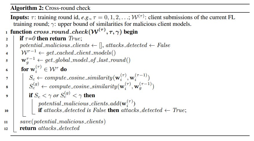Table of Links Abstract and Introduction Problem Setting The Proposed Two-Stages Anomaly Detection Verifiable Anomaly Detection using ZKP Evaluations Related Works Conclusion & References 3 THE PROPOSED TWO-STAGED ANOMALY DETECTION 3.1 CROSS-ROUND CHECK The goal of the cross-round check is to detect whether attacks happened in the current FL iteration. Below, we first give a high-level idea of the algorithm, then explain the algorithm in more details. The cross-round check algorithm is given in Algorithm 2, which has the following steps. The server loads the reference models, including the global model from the last FL training round, as well as the cached local models that are deemed as “benign” from the previous FL training round (Line 4 and 5). For the first round that does not have a reference global model and cached local models, the algorithm assumes there are attacks and skips the cross-round check stage to directly go into the second stage. Step 1: Initialization. If any client models are detected as “potentially malicious”, the server outputs an indicator that attacks might have happened in the current FL round, and the algorithm then enters the next stage to further inspect and remove malicious client models. Step 3: Return an indicator of potential attacks. 3.2 CROSS-CLIENT ANOMALY DETECTION We give an overview of the cross-client detection stage and provide details of the algorithm. Overview. In cross-client detection, the server utilizes the three sigma rule to further determine whether attacks have indeed happened on the potentially malicious clients determined in the first stage. Only those local models that are again flagged as “malicious” at this stage are removed from the aggregation. In each FL iteration, the server computes an L2 score between each local model and an approximate average model. The server then uses these scores to compute an approximate normal distribution. Based on the three sigma rule, the server computes a bound for filtering out potentially malicious client models. The algorithm is shown in Algorithm 3. Below, we explain the algorithm in steps. Our algorithm takes the global model computed after removing all malicious local models in the last round as the average model for the current FL round. For the first FL training round that does not have an average model for reference, our algorithm uses mKrum to compute an approximate average model. As the FL server does not know the number of potential malicious clients, we set m to L/2 to compute an approximate average model based on the assumption that the number of malicious clients is less than L/2, where L is the number of clients in each FL round. Such an approximate average model is used to compute L2 distances for local models in the current FL training round. Step 1: Obtain an average model. The algorithm utilizes the average model, denoted as w , and uses it to compute an 2 score ( ., the Euclidean distance) for each local model w as S = ||wiI − w || in the current FL training round. Step 2: Compute scores for each client model. avg L i.e i i avg The bound for removing malicious clients is defined as λ (λ > 0) standard deviation of the mean as µ + λσ. The server deems local models with scores higher than the boundary as “anomaly local models” and removes them from the aggregation. Note that we only take one side of the bounds of the three sigma rule, as we prefer lower L2 scores, which indicate that the local model is “closer” to the average model. Thus, we do not filter out client models with scores lower than µ − λσ. Step 4: Remove malicious local models based on the three sigma rule and the L2 scores. Step 5: Compute a new average model for later FL iteration. After removing malicious client models, the server uses the benign local models to compute an average model for the next round. Algorithm 2 and Algorithm 3 utilize local models and global models to compute scores (i.e., cosine similarities in Algorithm 2 and L2 distances in Algorithm 3), which requires storing full client models in cache and use them in computation. To reduce the cache size and the computation time, similar to Fung et al. (2020), we utilize a layer that can represent a whole model, called the “importance layer”, instead of using full models. Intuitively, we select the second-to-the-last layer, as it contains more information in regards to the whole model. We experimentally verify this in Section 5. Optimizations for computation and storage.

Augmentastic || Augmented Reality

Too Long; Didn't Read

Discover Saakuru: Web3 Mass-Adoption with 0-FEES

The Proposed Two-Stages of Zero-Knowledge-Proof-Based Anomaly Detection

Too Long; Didn't Read

Company Mentioned

Quantification Theory Research Publication

About Author

TOPICS

THIS ARTICLE WAS FEATURED IN...

The Proposed Two-Stages of Zero-Knowledge-Proof-Based Anomaly Detection

Too Long; Didn't Read

Company Mentioned

Quantification Theory Research Publication

About Author

TOPICS

THIS ARTICLE WAS FEATURED IN...

RELATED STORIES