paint-brush
Streamlining R1CS Normalization: A Guide to the Normalization Algorithmby@escholar

Streamlining R1CS Normalization: A Guide to the Normalization Algorithm

tldt arrow

Too Long; Didn't Read

The R1CS normalization algorithm facilitates standardized representations of blockchain data through data flow graphs and constraint generation techniques. This guide explores the intricate steps involved, highlighting their role in enhancing blockchain efficiency and scalability, and advancing the field of cryptography and blockchain technology.
featured image - Streamlining R1CS Normalization: A Guide to the Normalization Algorithm
EScholar: Electronic Academic Papers for Scholars HackerNoon profile picture

Authors:

(1) Chenhao Shi, Shanghai Jiao Tong University;

(2) Ruibang Liu, Shanghai Jiao Tong University;

(3) Guoqiang Li†, Shanghai Jiao Tong University.

Table of Links

Abstract & Introduction

Preliminaries

Normalization Algorithm

Evaluation

Conclusion & References

III. NORMALIZATION ALGORITHM

In this section, we formally introduce various steps of the normalization generation algorithm and several data structures defined within the algorithm.


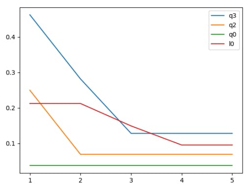
Fig. 8. The convergence process of each node.


A. Construction of RNode Graph


Our study presents a novel data structure, RNode, that represents variable relationships within an R1CS arithmetic circuit. This structure, RNode, facilitates efficient problem-solving by tracking interconnections among variables, which is formally defined as follows,


Definition III.1. An RNode is a node of two types in the data flow graph constructed in this normalization algorithm.


RNode = ConstNode ∪ V arNode

ConstNode = {ConstV alue, Operation, F ather, Child}

V arNode = {Operation, F ather, Child}


where


∀c is a ConstNode ∩ c.Operation = Null, c.child = ∅

∀c is a ConstNode ∩ c.Operation ∈ {Add, Mul}, c.f ather = ∅


RNodes can be categorized into two types based on the variables they represent. The first category represents the original variables in the solution vector of the R1CS and the intermediate variables produced during the construction of the arithmetic circuit. The second category represents the constants in the data flow graph. Each RNode includes both an operator and a computed result, which store the calculation method between its two parent nodes and represent the calculated result of the subtree rooted in itself.


The generation of the RNode Graph involves 3 main stages:


  1. Transform each constraint into an equation of a ∗ b = c, as required by the R1CS constraints.


2) Convert each constraint in the original R1CS constraint into an equation.


3) Organize the resulting equations containing common sub-expressions into a DAG-structured expression tree.


The core logic of the RNode Graph generation algorithm is similar to the procedure we previously mentioned for constructing the RNode Graph.


The RNode is a data structure used to store information about the variables in an R1CS during the construction of the RNode Graph. Unlike typical nodes in an expression tree, each RNode stores information about both the variable and operator involved in a given operation, allowing each operator’s output to be considered an intermediate variable and making it more closely aligned with the properties of an R1CS constraint set.


In practice, the merging and splitting of constraints poses a challenge in determining the equivalence of R1CS constraint sets. However, our RNode graph generation algorithm has observed that this merging or splitting does not lead to substantial differences. When constraints are merged, one variable is subtracted from the original constraint set. For instance, the merging process can be exemplified by the following example.


However, the subtracted variable will be added back into the RNode Graph as an intermediate node in the sum-product expression during the construction of the RNode Graph. The reverse is also true.


Further abstraction of the RNode Graph is required to eliminate the difference observed in the graphs generated by equivalent R1CS due to the different variable ordering in the constraint set. The main difference is observed in the order of addition in constructing the expression of continuous addition. At this stage, we do not have sufficient information to determine the sequential execution order. During the algorithm execution flow, two variables are randomly selected and added together, resulting in a different structure in the graph.


B. Tile Selection


Here, we categorize tiles into three types and give the formal definition of tile.


Definition III.2. Tile is a tree-like subgraph of the RNode Graph, representing a constraint in R1CS.


  1. Quadratic: Tiles with the form x ∗ y = z, where x, y, and z are variables.


  2. MulLinear: Tiles whose root is obtained by multiplying its two parents, with at least one of the parents being a constant.


3) AddLinear: Tiles whose root is obtained by adding its two parents.


Tile is essentially a set of linear equations generated by applying certain constraints to variables in the R1CS. We can use tiles as building blocks to construct a normalized R1CS that is both correct and scalable.


During tile selection, we divide the data flow graph from the previous step into 3 types. While AddLinear and MulLinear tiles are generated by linear constraints and are essentially linear tiles, their logical processing differs significantly. Hence, we discuss them as two separate types.


  1. We temporarily put aside the constraint merging step until we obtain more information about the tree in subsequent steps.


  2. If there is a need to generate merged formulas later, it can be achieved simply by applying a fixed algorithm to the unmerged formulas.


  3. The implementation of the tile selection algorithm is relatively simple.


When the RNode graph is generated, we select a node with no successors and use it as the root to partition a subgraph from the RNode Graph as a tile. We then remove this tile from the RNode Graph and repeat this loop until the entire graph is partitioned. Detailed code will posted in github.


The difference between data flow graphs generated by equivalent R1CS constraint systems lies in the order of node additions when processing linear tiles. However, the nodes added within a linear constraint, when considered as a set, are equivalent. This implies that the different addition order only affects the traversal order of the nodes. Therefore, if we consider the selected linear tiles as the products of the selected nodes and their respective coefficients, the chosen sets of linear tiles from equivalent R1CS constraint systems are the same. In other words, there is no distinction between the selected sets of tiles for equivalent R1CS constraint systems. Revised paragraph: The difference between data flow graphs generated by equivalent R1CS constraint systems lies in the order of node additions when processing linear tiles. However, the nodes added within a linear constraint, when considered as a set, are equivalent. This implies that the different addition order only affects the traversal order of the nodes. Therefore, the selected sets of linear tiles from equivalent R1CS constraint systems are the same if we consider the selected linear tiles as the products of the selected nodes and their respective coefficients. In other words, there is no distinction between the selected sets of tiles for equivalent R1CS constraint systems.


C. Graph Abstraction


We further abstract the data flow graph based on the selected tiles to eliminate the differences between various equivalent R1CS constraint systems. Specifically, we abstract linear tiles using a new node. By doing so, we mask the difference in addition order within linear tiles in the RNode Graph and transform the relationship between external nodes and specific nodes within the linear tile into a relationship between external nodes and the tile to which the particular node belongs. In this abstracted data flow graph, the types of edges are as follows:


  1. Non-linear tile abstract node to non-linear tile abstract node: The two vertices already existed in the original RNode graph. This edge type remains consistent with the original RNode graph.


2) Non-linear tile abstract node to linear tile abstract node: This edge type exists only if there are non-abstract nodes in the linear tile represented by the abstract node.


3) Linear tile abstract node to linear tile abstract node: This edge type exists only if the two abstract nodes represent linear tiles that share common non-abstract nodes.


D. Tile Weight Calculation


In this step, we use the Weighted PageRank algorithm to calculate the scores of each vertex in the data flow graph.


The previous steps eliminated the differences in the data flow graphs generated by equivalent R1CS through the abstraction of linear tiles. In the following step, constraints are generated on a tile-by-tile basis, and a criterion for tile order is proposed to sort the generated constraints.


In the algorithm proposed in this paper, the Weighted PageRank algorithm is used to calculate the weights of each node in the abstracted data flow graph, which are then used as the basis for calculating the weights of the corresponding constraints for each tile. Compared to the traditional PageRank algorithm, this algorithm assigns weights to every edge in the graph and adjusts the iterative formula for node weights. In the Weighted PageRank algorithm, as mentioned in the former section, the formula for calculating node scores is defined as follows:


In this algorithm, the primary purpose of using the Weighted PageRank algorithm is to reduce the symmetry of the abstracted data flow graph. The structure of the graph is significantly simplified in the previous step through the simplification of linear tiles. However, some structures in the graph still contain symmetric nodes. If general algorithms are used to calculate the weights of nodes, these symmetric nodes may be assigned the same weight, which can lead to problems in subsequent constraint generation and sorting. To address this issue, the Weighted PageRank algorithm is employed to calculate weights for different nodes. This helps increase the asymmetry of the graph and minimize the occurrence of nodes with the same score.


In this algorithm, the iterative formula for scores in the Weighted PageRank algorithm is further adjusted. The node weights retained in the original data flow graph are set to 1, while for nodes abstracted from linear constraints, their weights are calculated through a series of steps.


Fig. 9. Two equivalent expressions of a quadratic constraint.


Finally, the variance of the normalized coefficients is utilized as the weight of the abstract node representing the linear constraint.


In this algorithm, the iterative formula for the node score in the Weighted PageRank algorithm is given by:


The scores for each node are calculated to determine the ranking of each constraint in the R1CS form.


E. Constraint Generation


In this step, we generate constraints in descending order of weight, with tiles as the unit, starting with quadratic constraints and followed by linear constraints.


In this phase, a portion of the variable ordering was determined through the quadratic tile. In the tripartite matrix group of the R1CS paradigm, the three-row vectors corresponding to quadratic constraints each have only one non-zero coefficient. Still, in matrices A and B, the two-row vectors corresponding to the same constraint are equivalent in the constraint representation, consistent with the commutativity of multiplication. This results in two equivalent expressions for the same quadratic constraint. Figure 9 illustrates an example of equivalent terms for a quadratic constraint.


In the abstract data flow graph, all vertices representing variables appearing in quadratic constraints are retained, making it possible to determine the choice of non-zero coefficients in the corresponding row vectors of matrices A and B in the tripartite matrix group of the R1CS paradigm based on the weights of each variable. The variables with higher weights are assigned to matrix A and given smaller indices in the variable mapping. The sorting rules for the ordering of variables that appear in quadratic constraints can be summarized as follows:


  1. Sort variables based on the highest weight value among all quadratic constraints in which they appear, such that variables with higher weight values have smaller indices in the variable mapping.


2) For variables that appear in the same constraint and have the same highest weight value sort them based on their scores in the Weighted PageRank algorithm for the nodes in the data flow graph corresponding to the variables. Variables with higher node scores will have smaller indices in the variable mapping and be assigned to the corresponding row vector in matrix A of the tripartite matrix group.


F. Adjustment of Linear Constraints


At this stage, the partition and ordering of constraints within a constraint group have been established, and the ordering of variables that appeared in quadratic constraints has also been determined. However, it is necessary to adjust the order of newly introduced variables in linear tiles in this step. As the example below demonstrates, introducing multiple new variables within a linear tile can result in disorderly sorting. This is because, in the previous actions, the specific structures of linear tile constraints were abstracted to eliminate differences in the RNode Graph.


Therefore, we introduce a new method to order the newly introduced variables in linear tiles. For each new variable introduced in a linear tile, its weight is calculated as


The new variables are sorted based on their weights. If the weights are the same, the coefficients of the variable in its linear tile are considered for comparison. The appearance of new variables in other linear tiles, to some extent, reflects their importance in the entire constraint group. Additionally, suppose certain new variables only appear in their constraints. In that case, their weights will be zero, and their ordering will only affect the constraints generated by their linear tile without changing the ordering of other constraints. Therefore, they can be sorted in descending order based on their coefficients alone.


This paper is available on arxiv under CC BY 4.0 DEED license.