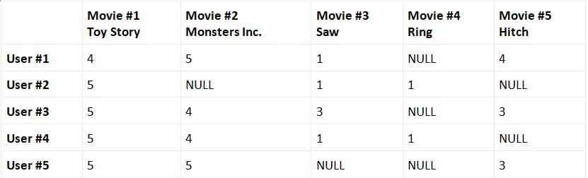
Principal Component Analysis — Unsupervised Learning Model

Learn how to train and evaluate an unsupervised machine learning model — principal component analysis in this article by Jillur Quddus, a lead technical architect, polyglot software engineer and data scientist. There are numerous real-world use cases, where the number of features available, which may potentially be used to train a model, is very large. A common example is economic data and using its constituents, stock price data, employment data, banking data, industrial data, and housing data together to predict the ( ). Such types of data are said to have high dimensionality. Though they offer numerous features that can be used to model a given use case, high-dimensional datasets increase the computational complexity of machine learning algorithms and more importantly may also result in over fitting. gross domestic product GDP Over fitting is one of the results of the , which formally describes the problem of analyzing data in high-dimensional spaces (which means that the data may contain many attributes, typically hundreds or even thousands of dimensions/features) but where that analysis no longer holds true in a lower-dimensional space. curse of dimensionality Informally, it describes the value of additional dimensions at the cost of model performance. ( ) is an technique used to preprocess and reduce the dimensionality of high-dimensional datasets while preserving the original structure and relationships inherent to the original dataset so that machine learning models can still learn from them and be used to make accurate predictions. Principal component analysis PCA unsupervised Movie recommendation system To better understand PCA, let’s study a movie recommendation use case. Our aim is to build a system that can make personalized movie recommendations to users based on historic user-community movie ratings. The historic user-community movie ratings data that we will use for our case study has been downloaded from GroupLens, a research laboratory based at the University of Minnesota that collects movie ratings and makes them available for public download at . For the purposes of this case study, we have transformed the individual and datasets into a single pivot table where the 300 rows represent 300 different users, and the 3,000 columns represent 3,000 different movies. https://grouplens.org/datasets/movielens/ movies ratings This transformed, pipe-delimited dataset can be found in the GitHub repository at . You can also find the code file for this article at . https://github.com/PacktPublishing/Machine-Learning-with-Apache-Spark-Quick-Start-Guide/tree/master/Chapter05/data/movie-ratings-data and is called movie-ratings-data/user-movie-ratings.csv https://github.com/PacktPublishing/Machine-Learning-with-Apache-Spark-Quick-Start-Guide/blob/master/Chapter05/chp05-02-principal-component-analysis.ipynb A sample of the historic user-community movie ratings dataset that we will study looks as follows: In this case, each movie is a different feature (or dimension) and each different user is a different instance (or observation). This sample table, therefore, represents a dataset containing 5 features. However, our actual dataset contains 3,000 different movies and therefore 3,000 features/dimensions. Furthermore, in a real-life representation, not all users would have rated all the movies, so there will be a significant number of missing values. Such a dataset, and the matrix used to represent it, is described as . These issues would pose a problem for machine learning algorithms, both in terms of computational complexity and the likelihood of over fitting. sparse To solve this problem, take a closer look at the previous sample table. It seems that users that rated Movie #1 highly (Toy Story) generally also rated Movie #2 highly (Monsters Inc.) as well. We could say, for example, that User #1 is of all fans of computer-animated children’s films, and so we could recommend to User #2 the other movies that User #1 has historically rated highly (this type of recommendation system where we use data from other users is called ). representative collaborative filtering At a high level, this is what PCA does — it identifies , called , within a high-dimensional dataset so that the dimensions of the original dataset can be reduced while preserving its underlying structure and still be representative in dimensions! These reduced datasets can then be fed into machine learning models to make predictions as normal, without the fear of any adverse effects from reducing the raw size of the original dataset. Our formal definition of PCA can therefore now be extended so that we can define PCA as the identification of a linear subspace of lower dimensionality where the largest variance in the original dataset is maintained. typical representations principal components lower Returning to our historic user-community movie ratings dataset, instead of eliminating Movie #2 entirely, we could seek to create a new feature that combines Movie #1 and Movie #2 in some manner. Extending this concept, we can create new features where each new feature is based on all the old features, and thereafter order these new features by how well they help us in predicting user movie ratings. Once ordered, we can drop the least important ones, thereby resulting in a reduction in dimensionality. So how does PCA achieve this? It does so by performing the following steps: 1. First, we standardize the original high-dimensional dataset. 2. Next, we take the standardized data and compute a covariance matrix that provides a means to measure how all our features relate to each other. 3. After computing the covariance matrix, we then find its and corresponding . Eigenvectors represent the principal components and provide a means to understand the direction of the data. Corresponding eigenvalues represent how much variance there is in the data in that direction. eigenvectors eigenvalues 4. The eigenvectors are then sorted in descending order based on their corresponding eigenvalues, after which the top eigenvectors are selected representing the most important representations found in the data. k 5. A new matrix is then constructed with these eigenvectors, thereby reducing the original -dimensional dataset into reduced dimensions. k n k Covariance matrix In mathematics, refers to a measure of how spread out a dataset is and is calculated by the sum of the squared distances of each data point, , from the mean , divided by the total number of data points, . This is represented by the following formula: variance xi x-bar N refers to a measure of how strong the correlation between two or more random variables is (in our case, our independent variables) and is calculated for variables and over dimensions: Covariance x y i If the covariance is positive, this implies that the independent variables are positively correlated. If the covariance is negative, this implies that the independent variables are negatively correlated. Finally, a covariance of zero implies that there is no correlation between the independent variables. Here, we are computing the covariance between all variables. A is a symmetric square matrix where the general element ( , ) is the covariance, , between independent variables and (which is the same as the symmetric covariance between and ). Note that the diagonal in a covariance matrix actually represents just the between those elements, by definition. covariance matrix i j cov(i, j) i j j i variance The covariance matrix is shown in the following table: Identity matrix An identity matrix is a square matrix in which all the elements along the main diagonal are 1 and the remaining elements are 0. Identity matrices are important for when we need to find all of the eigenvectors for a matrix. For example, a 3 x 3 identity matrix looks as follows: Eigenvectors and eigenvalues In linear algebra, eigenvectors are a special set of vectors whose remains unchanged when a linear transformation is applied to it, and only changes by a factor. In the context of dimensionality reduction, eigenvectors represent the principal components and provide a means to understand the direction of the data. direction scalar Consider a matrix, , of dimensions ( x ). We can multiply by a vector, (of dimensions x 1 by definition), which results in a new vector, (of dimensions x 1), as follows: A m n A x n b m In other words, However, in some cases, the resulting vector, , is actually a scaled version of the original vector, . We call this scalar factor , in which case the formula above can be rewritten as follows: b x λ We say that is an of matrix , and is an associated with . In the context of dimensionality reduction, eigenvalues represent how much variance there is in the data in that direction. λ eigenvalue A x eigenvector λ In order to find all the eigenvectors for a matrix, we need to solve the following equation for each eigenvalue, where is an identity matrix with the same dimensions as matrix : I A Once all of the eigenvectors for the covariance matrix are found, these are then sorted in descending order by their corresponding eigenvalues. Since eigenvalues represent the amount of variance in the data for that direction, the first eigenvector in the ordered list represents the principal component that captures the most variance in the original variables from the original dataset, and so on. For example, as illustrated in the figure below, if we were to plot a dataset with two dimensions or features, the first eigenvector (which will be the first principal component in order of importance) would represent the direction of most variation between the two features. The second eigenvector (the second principal component in order of importance) would represent the direction of second-most variation between the two features: To help choose the number of principal components, , to select from the top of the ordered list of eigenvectors, we can plot the number of principal components on the axis against the cumulative explained variance on the axis, as illustrated in the next figure, where the explained variance is the ratio between the variance of that principal component and the total variance (that is, the sum of all eigenvalues): k x y Using this as an example, we would select around the first 300 principal components, as these describe the most variation within the data out of the 3,000 in total. Finally, we construct a new matrix by projecting the original dataset into -dimensional space represented by the eigenvectors selected, thereby reducing the dimensionality of the original dataset from 3,000 dimensions to 300 dimensions. This preprocessed and reduced dataset can then be used to train machine learning models as normal. k PCA in Apache Spark Let’s now return to our transformed pipe-delimited user-community movie ratings dataset, , which contains ratings by 300 users covering 3,000 movies. We will develop an application in Apache Spark that seeks to reduce the dimensionality of this dataset while preserving its structure using PCA. To do this, we will go through the following steps: movie-ratings-data/user-movie-ratings.csv 1. First, let’s load the transformed, pipe-delimited user-community movie ratings dataset into a Spark dataframe using the following code. The resulting Spark dataframe will have 300 rows (representing the 300 different users) and 3,001 columns (representing the 3,000 different movies plus the user ID column): user_movie_ratings_df = sqlContext.read .format('com.databricks.spark.csv').options(header = 'true', inferschema = 'true', delimiter = '|') .load(' print((user_movie_ratings_df.count(), len(user_movie_ratings_df.columns))) 2. We can now generate feature vectors containing 3,000 elements (representing the 3,000 features) using 's , as we have seen before. We can achieve this using the following code: MLlib MLlib VectorAssembler feature_columns = user_movie_ratings_df.columns feature_columns.remove('userId') vector_assembler = VectorAssembler(inputCols = feature_columns, outputCol = 'features') user_movie_ratings_features_df = vector_assembler .transform(user_movie_ratings_df) .select(['userId', 'features']) 3. Before we can reduce the dimensionality of the dataset using PCA, we first need to standardize the features that we described previously. This can be achieved using 's estimator and fitting it to the Spark dataframe containing our feature vectors, as follows: MLlib StandardScaler standardizer = StandardScaler(withMean=True, withStd=True, inputCol='features', outputCol='std_features') standardizer_model = standardizer .fit(user_movie_ratings_features_df) user_movie_ratings_standardized_features_df = standardizer_model.transform(user_movie_ratings_features_df) 4. Next, we convert our scaled features into an instance. A is a distributed matrix with no index, where each row is a vector. We achieve this by converting our scaled features data frame into an RDD and mapping each row of the RDD to the corresponding scaled feature vector. We then pass this RDD to 's (as shown in the following code), resulting in a matrix of standardized feature vectors of dimensions 300 x 3,000: MLlibRowMatrix RowMatrix MLlib RowMatrix() scaled_features_rows_rdd = user_movie_ratings_standardized_features_df .select("std_features").rdd scaled_features_matrix = RowMatrix(scaled_features_rows_rdd .map(lambda x: x[0].tolist())) 5. Now that we have our standardized data in matrix form, we can easily compute the top principal components by invoking the method exposed by 's . We can compute the top 300 principal components as follows: k computePrincipalComponents() MLlib RowMatrix number_principal_components = 300 principal_components = scaled_features_matrix .computePrincipalComponents(number_principal_components) 6. Now that we have identified the top 300 principal components, we can project the standardized user-community movie ratings data from 3,000 dimensions to a linear subspace of only 300 dimensions while preserving the largest variances from the original dataset. This is achieved by using matrix multiplication and multiplying the matrix containing the standardized data by the matrix containing the top 300 principal components, as follows: projected_matrix = scaled_features_matrix .multiply(principal_components) print((projected_matrix.numRows(), projected_matrix.numCols())) The resulting matrix now has dimensions of 300 x 300, confirming the reduction in dimensionality from the original 3,000 to only 300! We can now use this projected matrix and its PCA feature vectors as the input into subsequent machine learning models as normal. 7. Alternatively, we can use 's estimator directly on the dataframe containing our standardized feature vectors to generate a new dataframe with a new column containing the PCA feature vectors, as follows: MLlib PCA() pca = PCA(k=number_principal_components, inputCol="std_features", outputCol="pca_features") pca_model = pca.fit(user_movie_ratings_standardized_features_df) user_movie_ratings_pca_df = pca_model .transform(user_movie_ratings_standardized_features_df) Again, this new dataframe and its PCA feature vectors can then be used to train subsequent machine learning models as normal. 8. Finally, we can extract the explained variance for each principal component from our PCA model by accessing its attribute as follows: explainedVariance pca_model.explainedVariance The resulting vector (of 300 elements) shows that, in our example, the first eigenvector (and therefore the first principal component) in the ordered list of principal components explains 8.2% of the variance; the second explains 4%, and so on. In this example, we have demonstrated how we can reduce the dimensionality of the user-community movie ratings dataset from 3,000 dimensions to only 300 dimensions while preserving its structure using PCA. The resulting reduced dataset can then be used to train machine learning models as normal, such as a hierarchical clustering model for collaborative filtering. If you found this article interesting, you can explore Machine Learning with Apache Spark Quick Start Guide to combine advanced analytics including machine learning, deep learning neural networks and natural language processing with modern scalable technologies including apache spark to derive actionable insights from big data in real-time. Machine Learning with Apache Spark Quick Start Guide can help you become familiar with advanced techniques for processing a large volume of data by applying machine learning algorithms.