paint-brush
Comparative Analysis: Learned Heuristics vs. WalkSAT in SAT Problem Solvingby@heuristicsearch

Comparative Analysis: Learned Heuristics vs. WalkSAT in SAT Problem Solving

tldt arrow

Too Long; Didn't Read

Dive deeper into the supplementary materials providing insights into intra-episode behavior, generalization across small and hard instances, and comparative analysis of learned SAT heuristics against the WalkSAT algorithm. Explore detailed tables, plots, and performance metrics for a comprehensive understanding of the evaluation outcomes. TLDR for Supplementary Materials: The supplementary materials offer detailed analysis on intra-episode behavior, generalization capabilities on small and hard instances, and a comparative evaluation of learned SAT heuristics versus the WalkSAT algorithm. Access additional tables, plots, and performance metrics for a comprehensive view of the evaluation results.
featured image - Comparative Analysis: Learned Heuristics vs. WalkSAT in SAT Problem Solving
Aiding in the focused exploration of potential solutions. HackerNoon profile picture

Authors:

(1) Ankur Nath, Department of Computer Science and Engineering, Texas A&M University;

(2) Alan Kuhnle, Department of Computer Science and Engineering, Texas A&M University.

Abstract & Introduction

Related work

Evaluation for Max-Cut

Evaluation for SAT

Summary and Outlook, References

Supplementary Materials

SUPPLEMENTARY MATERIALS

Reproducibility

We use the publicly available implementation of ECO-DQN[2] and GNNSAT[3] as our code base. To ensure a fair comparison, we employ the pretrained models from the original papers. However, for S2V-DQN applied to ER graphs with |V | = 60, we conduct training from scratch due to the inability to load the pretrained model with the hyperparameters provided in the original paper. We provide all our experimental results, code, and data at this link[4].


For training skewed graphs for the Max-Cut problem, we adopt the hyperparameters outlined in the original paper and modify the dataset while keeping other settings intact.


Experimental Setup We run all experiments on two NVIDIA RTX A4000 (16GB memory) GPUs with Intel Xeon(R) w5-2445 CPUs at 3.10 GHz and 64 GB of memory

Additional Tables and Plots

In this section, you can find the tables and plots omitted in the main paper due to space constraints.

Intra-episode Behavior

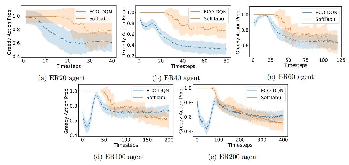
Figure 4 and 5 present an analysis of the intra-episode behavior of ECO-DQN and SoftTabu agents across a diverse range of distributions.


Figure 4: Intra-episode behavior of ECO-DQN and SoftTabu agents averaged across all 100 instances from the validation set of ER graphs with from |V | = 20 to 200.

Generalisation on Small Instances

Understanding the generalization of agents is crucial, as it determines their practical utility in real world applications where the data distribution may vary or evolve over time. Table 4 and 5 provide detailed analysis of how well these agents can adapt and perform in scenarios that go beyond their training data.


Figure 5: Intra-episode behavior of ECO-DQN and SoftTabu agents averaged across all 100 instances from the validation set of BA graphs with from |V | = 20 to 200.


Table 4: Generalisation of agents trained on ER graphs of size |V | = 40 to unseen graph sizes and structures.


Table 5: Generalisation of agents trained on BA graphs of size |V | = 40 to unseen graph sizes and structures.


Generalisation on Hard Instances and Real World Datasets

Table 6 presents a performance analysis of agents that have been trained on skew graphs, specifically those with |V | = 200. The primary focus is on how these agents perform when faced with established benchmark tasks, with the best-performing results being emphasized and displayed in bold for clarity.


Table 6: Average performance of agents trained on skew graphs of size |V | = 200 on known benchmarks (best in bold).


Distributions of Actions on Hard Instances

Figure 6: Distribution of flips (number of times a vertex state is changed during an episode) of SoftTabu agents in descending order on a random graph from three distributions with |V | = 2000 from GSET Dataset, Trained on ER with |V | = 200. We limit the number of vertices to 25.


Figure 7: Score of SoftTabu agents on a random graph from three distributions with |V | = 2000 from GSET Dataset, Trained on ER with |V | = 200.

Evalution of SAT

In Table 7, we compare the performance of learned heuristics alongside the WalkSAT algorithm. For WalkSAT, we have set the value of the parameter p to 0.5, following the experimental setup used in GNNSAT. Additionally, we have fine-tuned the algorithm to determine the optimal p value.


Table 7: Performance of the learned heuristics and WalkSAT. For WalkSAT, we set the value of p = 0.5 following the experimental setup of GNNSAT and also tune the algorithm for the optimal value. In each cell, there are three metrics (from top to bottom): the ratio of the average number of steps, the median number of steps, and the percentage solved. *Values as reported in GNNSAT for reference.


[2] Code available at: https://github.com/tomdbar/eco-dqn

[3] Code available at: https://github.com/emreyolcu/sat

[4] Code available at: https://tinyurl.com/52ykxtaj


This paper is available on arxiv under CC 4.0 DEED license.