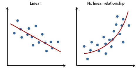
Linear Regression and its Mathematical implementation

What is Linear Regression ?

Linear regression is a predictive statistical approach for modelling relationship between a dependent variable with a given set of independent variables.

It is a linear approach to modeling the relationship between a dependent variable and one or more independent variables. When we have only one independent variable it is as called simple linear regression. For more than one independent variable, the process is called as multiple linear regression.

Linear Regression Model Representation

Linear Regression representation consists of a linear equation that combines a specific set of input values (x), the solution to which is the predicted output (y) for that set of input values (y).

The linear equation assigns one scale factor to each input value or column, called a coefficient and represented by the capital Greek letter Beta (B). One additional coefficient is also added, giving the line an additional degree of freedom (e.g. moving up and down on a two-dimensional plot) and is often called the intercept or the bias coefficient.

For example, in a simple regression problem (a single x and a single y), the form of the model would be:

y = B0 + B1*x, where

1. B0 - represents the intercept
2. B1 - represents the coefficient
3. x - represents the independent variable
4. y - represents the output or the dependent variable

In higher dimensions when we have more than one input (x), the line is called a plane or a hyper-plane. The representation therefore is the form of the equation and the specific values used for the coefficients (e.g. B0 and B1 in the above example).

The General equation for a Multiple linear regression with p - independent variables looks like this:

Ordinary Least Squares

When we have more than one input we can use Ordinary Least Squares to estimate the values of the coefficients.

The Ordinary Least Squares procedure seeks to minimize the sum of the squared residuals. This means that given a regression line through the data we calculate the distance from each data point to the regression line, square it, and sum all of the squared errors together. This is the quantity that ordinary least squares seeks to minimize.

Gradient Descent

When there are one or more inputs, you can use a process of optimizing the values of the coefficients by iteratively minimizing the error of the model on your training data. This process is called as Gradient Descent.

It works by starting with random values for each coefficient. The sum of the squared errors are calculated for each pair of input and output values. A learning rate is used as a scale factor and the coefficients are updated in the direction towards minimizing the error. The process is repeated until a minimum sum squared error is achieved or no further improvement is possible.

Application of Linear Regression

1. Studying engine performance from test data in automobiles.
2. Least squares regression is used to model causal relationships between parameters in biological systems.
3. OLS (ordinary least squares) regression is be used in weather data analysis.
4. Linear regression is be used in market research studies and customer survey results analysis.
5. Linear regression is used in observational astronomy. A number of statistical tools and methods are used in astronomical data analysis, and there are entire libraries in languages like Python meant to do data analysis in astrophysics..