Authors: (1) Davide Viviano, Department of Economics, Harvard University; (2) Lihua Lei, Graduate School of Business, Stanford University; (3) Guido Imbens, Graduate School of Business and Department of Economics, Stanford University; (4) Brian Karrer, FAIR, Meta; (5) Okke Schrijvers, Meta Central Applied Science; (6) Liang Shi, Meta Central Applied Science. Table of Links Abstract & Introduction Setup (When) should you cluster? Choosing the cluster design Empirical illustration and numerical studies Recommendations for practice References A) Notation B) Endogenous peer effects C) Proofs 5 Empirical illustration and numerical studies In this section we illustrate the properties of the procedure in two empirical applications, one using unique data from the Facebook friendship and messaging graphs, and one using data from an experiment conducted in rural China by Cai et al. [2015]. We provide further evidence supporting our theoretical analysis using simulated networks in Section 5.3. 5.1 Clustering on Facebook graphs We first study the procedure’s properties for two clustering algorithms implemented at scale on social networks owned by Meta: Louvain algorithm [Blondel et al., 2008], Balanced Partitioning [Kabiljo et al., 2017]. We consider two graphs owned by Meta. In each graph, edges are continuous variables. In the first graph, edges capture the strength of the friendship in the Facebook graph, and in the second graph they capture connections based on messaging on Facebook, in both cases the data was aggregated and de-identified. We compute our statistics by setting the edges to be zero if below the 5th, 10th, and 50th percentile. We will refer to these graphs obtained as dense, moderate (mod), and sparse after thresholding (graphs all have a bounded maximum degree). We report the bias and variance, with the variance weighted by a parameter ξn, defined respectively as Louvain and Balanced Partitioning clustering produce a hierarchical clustering structure with a growing number of clusters. We consider three “types” of such algorithms, corresponding to three levels in the clustering structure hierarchy (i.e., different numbers of clusters), defined as Type 1, 2, and 3, respectively. For Louvain clustering, higher-order types denote more clusters, whereas it is the opposite for Balanced Partitioning. For each clustering, we report log(Kn/n), log-ratio of the number of clusters over the population size. Table 2 collects each of these algorithms’ worst-case bias and variance and the number of clusters per individual. Louvain algorithm dominates Balanced Partitioning both in worstcase variance and bias. A larger number of clusters increases the bias but decreases the variance, which we observe throughout all graphs. The bias increases for sparser networks because the denominator |Ni | decreases. 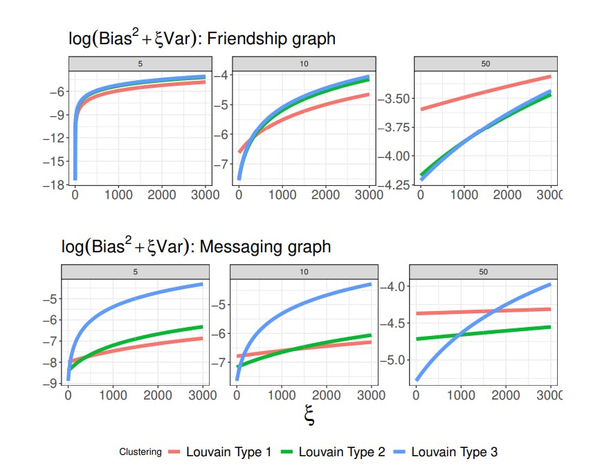Figure 3 reports the objective function for different graphs, Louvain algorithms, and degrees of sparsity. For ξn ≈ 1, the Louvain algorithm with the largest number of clusters (Type 3) dominates the other two algorithms in all but one case. This result provides some interpretable comparisons for the number of clusters. We also observe a trade-off between the number of clusters and the degree of sparsity of the adjacency matrix as ξn decreases. Louvain clustering with the largest number of clusters (Type 1) is optimal for a dense graph with ξn ≫ 1. Such clustering, however, is sub-optimal as the graph becomes more sparse. This result is intuitive: for denser networks, a larger number of clusters may best control the estimator’s bias relative to the bias induced by other clustering algorithms. These comparisons motivate trade-offs in the choice of the graph (and its density) and the clustering algorithm. We recommend practitioners compare clustering by averaging objective functions over different sparsity thresholding. For example, it is possible to compare clustering based on the average objective across different graphs using some priors on the degree of sparsity without affecting our theoretical results. Finally, note that using Theorem 3.6 it is possible to compute the smallest values of the spillover effects that would motivate using a cluster instead of Bernoulli design. From Theorem 3.6, researchers should prefer a cluster over a Bernoulli design if In summary, our results shed light on using clustering algorithms for large-scale implementation on online platforms. These results suggest that Louvain clustering with possibly many clusters performs best in practice. It confirms intuitive arguments in Karrer et al. [2021] who also recommend Louvain clustering based on AA-tests. 5.2 Clustering in the field We consider as an application the problem of informing individuals to increase insurance takeup studied in Cai et al. [2015]. The authors collected network information in approximately 184 villages in rural China from 48 larger regions. We use network data collected by Cai et al. [2015] to study the properties of the proposed method, where we assume that two individuals are connected if at least one of the two indicates the other as a friend. Because we do not require information from end-line outcomes, we construct a network using information from surveyed individuals as well as their friends. The network has in total 7649 nodes, once we also include individuals who are friends of surveyed individuals (but do not necessarily live in their same village or were surveyed in the experiment). Individuals between villages present on average 50% of their connections outside their village. On the other hand, individuals in different regions (with approximately 50 regions) have 99% of their connections within the same region. We use an adjacency matrix a “weak ties” adjacency matrix, where two individuals are connected if either indicates the other has a friend. We study clustering within each region and report results for different clustering algorithms. Clustering within each region is performed as in Algorithm 1, where we first estimate Xˆ (K) via semi-definite programming, use K-means algorithm to retrieve the clusters from Xˆ (K) and iterate to estimate the optimal number of clusters K. We report the frontier with respect to the absolute bias consistently with Algorithm 1. 5.2.1 How many clusters should we choose? Figure 4 presents the main results. The left-hand side panel reports the average number of estimated clusters, estimated by the proposed method divided by the population size in a given cluster. Different choices of ξn justify a different number of clusters. For ξn = 1, the number of clusters is 7%, the total population size, whereas for ξn = 15, the number of clusters is roughly half the population size. To gain further intuition of its practical implication, take ψ¯ = 0.24 approximately equal to the outcomes’ variance in Cai et al. [2015] and ϕ¯ n = 0.27 as in Table 2 in Cai et al. [2015]. A recommended choice of ξn is approximately ψ/¯ ϕ¯2 n = 3.29. This choice puts slightly more weight on the bias than the variance when λ = 1, and therefore can be considered a conservative choice for the number of clusters.[13] Even with such a conservative choice, the suggested number of clusters is large relative to the population size. In this case, the optimal number of clusters is around 15% of the overall population size, approximately 600 clusters with a surveyed sample size of 3600 individuals. This number is consistent (in scale) with the choice in the number of clusters in other applications in development, such as Egger et al. [2022], Alatas et al. [2012], but larger than the number of villages that we have in the application in Cai et al. [2015]. 5.2.2 Comparison with other clustering methods Next, we compare the procedure (denoted as “Causal Clustering”) with the following alternative clustering algorithms: ε-net clustering as in Eckles et al. [2017] with ε = 3 as suggested in Eckles et al. [2017]; spectral clustering with a fixed number of clusters equal to n/3, where n is the population size in a given region (note that spectral clustering do not optimize over the number of clusters); Louvain clustering with default parameters selected by the R-package igraph; clustering based on village identity of each individual (creating one additional cluster for those individuals whose village is missing in the data). We contrast the objective function with alternative algorithms in the right-hand side of Figure 4. The proposed method achieves the smallest objective function across all competitors, providing suggestive evidence that Algorithm 1 (with a semi-definite relaxation) works particularly well in practice. For a smaller number of clusters the method is closer to the Louvain clustering algorithm, while for a larger number of clusters the objective of the algorithm is close to the objective of the spectral algorithm. Interestingly, clustering based on village identity leads to the largest loss function. This is because individuals are connected within and between villages in this application. Finally, in Figure 5 (first three panels), we report the mean-squared error obtained by simulating the model in Cai et al. [2015] (Table 2, Column 4) and vary the variance of the residuals σ 2 ∈ {1/4, 1/2, 1} to emulate settings with high, medium and low signal to noise ratio. The model in Cai et al. [2015] assumes that individual outcomes depend on neighbors’ treatments, consistently with our Assumption 1. Our method uniformly outperforms competitors in terms of mean-squared error, except for the Louvain algorithm when the signal-to-noise ratio is particularly high, but not in the remaining settings. In the last panel, we consider settings where the local interference assumption is violated, and we calibrate our model to the specification in Cai et al. [2015] (Column 4, Table 5), where the individual outcome depends on the neighbors’ outcomes, violating Assumption 1 and introducing global dependence. We fix the residuals’ variance to be σ 2 = 1/4, whereas the results are robust as we increase σ 2 . In this setup, we observe a larger mean-squared error of all methods, with the proposed method achieving the lowest mean-squared error. 5.3 A numerical study Next, we illustrate the properties of the method in numerical studies. We consider three different data generating processes for the network formation: a geometric network formation, Albert Barabasi network and Erdos-Renyi graph. The geometric network takes the form Ai,j = 1{|Xi,1 − Xj,1|/2 +|Xi,2 − Xj,2|/2 ≤ rn} where rn = p 4/2.75n similarly to simulations in Leung [2020]. Here, Xi,1, Xi,2 are drawn independently from a uniform distribution between [−1, 1]. For the Albert-Barabasi network we first draw n/5 edges uniformly according to Erdos-Renyi graph with probabilities p = 10/n, and second, we draw sequentially connections of the new nodes to the existing ones with probability equal to the number of connection of each pre-existing node divided by the overall number of connections. Finally, the Erdos-Renyi graph is generated with probability of connection p = 2/n. We study the properties of the proposed method and of the same competitors discussed in Section 5.2. Figure 6 showcases that the proposed procedure leads to the lowest objective function. This result is consistent with our theoretical findings. Figure 7 showcases that the number of clusters increases in the sample size, varies substantially across different data generating processes, and increases in ξn. [13] This follows from the fact that ξn is proportional to ψ/¯ ϕ¯2 n for clusters whose bias is of order O(ϕ¯ n), and researcher’s goal is to minimize the worst-case mean squared error (λ = 1). This paper is under CC 1.0 license. available on arxiv

Too Long; Didn't Read

Questions about cloud security? Get answers here.

Design of Cluster Experiments: Empirical Illustration and Numerical Studies

Too Long; Didn't Read

EScholar: Electronic Academic Papers for Scholars

About Author

TOPICS

THIS ARTICLE WAS FEATURED IN...

Design of Cluster Experiments: Empirical Illustration and Numerical Studies

Too Long; Didn't Read

EScholar: Electronic Academic Papers for Scholars

About Author

TOPICS

THIS ARTICLE WAS FEATURED IN...

RELATED STORIES