paint-brush
Building Your AI Radiologist: A Fun Guide to Creating a Pneumonia Detector with VGG16by@kisican
541 reads
541 reads

Building Your AI Radiologist: A Fun Guide to Creating a Pneumonia Detector with VGG16

by Can KisiJuly 9th, 2024
Read on Terminal Reader
Read this story w/o Javascript

Too Long; Didn't Read

Radiology is a field that significantly depends on the expertise of highly skilled professionals.. This is where artificial intelligence (AI) steps in, transforming the field by enhancing human capabilities. By the end of this article, you'll have crafted your very own image classifier model to analyse and detect pneumonia in medical images!
featured image - Building Your AI Radiologist: A Fun Guide to Creating a Pneumonia Detector with VGG16
Can Kisi HackerNoon profile picture

Radiology is a field that significantly depends on the expertise of highly skilled professionals. Radiologists analyse medical images to diagnose and monitor a range of conditions, from simple fractures to complex diseases such as cancer. Yet, with the surge in medical imaging and the urgent need for fast, accurate diagnoses, radiologists are under tremendous pressure. This is where artificial intelligence (AI) steps in, transforming the field by enhancing human capabilities. By the end of this article, you'll have crafted your very own image classifier model to assist in detecting pneumonia in medical images.

Step 1: Setting Up Your Environment

Before diving into coding, we need to ensure our environment is ready. We'll start by installing the necessary libraries:

%pip install --upgrade tensorflow keras numpy pandas sklearn pillow


These libraries are essential for building and training our model:

  • tensorflow and keras for creating and training neural networks.
  • numpy for numerical operations.
  • pandas for data manipulation.
  • sklearn for preprocessing data.
  • pillow for image processing.

Step 2: Importing Libraries

With the libraries installed, let's import them:

import os
from tensorflow import keras
from tensorflow.keras.models import Sequential
from tensorflow.keras.layers import Dense, Conv2D, MaxPool2D, Flatten
from tensorflow.keras.preprocessing.image import ImageDataGenerator
import numpy as np


We start by importing several essential libraries and modules needed for building and training a neural network model for image processing tasks. We’ll be using TensorFlow and its submodules to create and manage our deep learning models. Specifically, we'll import Keras to use as our high-level API, Sequential for constructing a linear stack of layers, and modules like Dense, Conv2D, MaxPool2D, and Flatten to build and configure various neural network layers. Additionally, ImageDataGenerator will help us augment our image data, enhancing the model's ability to generalize. Lastly, we'll import numpy for its numerical operations support, particularly useful for handling arrays and performing mathematical functions.

Step 3: Preparing the Data

Our AI radiologist needs data to learn from. We'll use ImageDataGenerator to load and augment our training and validation data: to download the data, we will be using our open-source data friend Kaggle, go and download the labelled dataset from the link here.


In the context of supervised learning here, the labelled dataset will be the ground truth that the machine learning model is supposed to predict.

trdata = ImageDataGenerator()
traindata = trdata.flow_from_directory(directory="data-task1/train", target_size=(224, 224))
tsdata = ImageDataGenerator()
testdata = tsdata.flow_from_directory(directory="data-task1/val", target_size=(224, 224))


This code snippet sets up data generators for our training and validation datasets. Images are resized to 224x224 pixels, the standard input size for the VGG16 model.


Step 4: Building the VGG16 Model

Now comes the fun part: building the VGG16 model. VGG16 is a popular convolutional neural network (CNN) architecture known for its simplicity and effectiveness thanks to its unique architecture built mainly on 13 convolutional layers and 3 fully connected layers. What sets VGG16 apart is its use of small 3x3 convolutional filters within a deep network. This design captures intricate patterns in images while ensuring computational efficiency. Here’s how we create it:


model = Sequential()

model.add(Conv2D(input_shape=(224,224,3), filters=64, kernel_size=(3,3), padding="same", activation="relu"))
model.add(Conv2D(filters=64, kernel_size=(3,3), padding="same", activation="relu"))
model.add(MaxPool2D(pool_size=(2,2), strides=(2,2)))

model.add(Conv2D(filters=128, kernel_size=(3,3), padding="same", activation="relu"))
model.add(MaxPool2D(pool_size=(2,2), strides=(2,2)))

model.add(Conv2D(filters=256, kernel_size=(3,3), padding="same", activation="relu"))
model.add(MaxPool2D(pool_size=(2,2), strides=(2,2)))

model.add(Conv2D(filters=512, kernel_size=(3,3), padding="same", activation="relu"))
model.add(MaxPool2D(pool_size=(2,2), strides=(2,2)))

model.add(Conv2D(filters=512, kernel_size=(3,3), padding="same", activation="relu"))
model.add(MaxPool2D(pool_size=(2,2), strides=(2,2)))

model.add(Flatten())
model.add(Dense(units=4096, activation="relu"))
model.add(Dense(units=2, activation="softmax"))

model.summary()


Let’s break it down:

  • Conv2D layers: These are convolutional layers that learn to detect features like edges and textures.
  • MaxPool2D layers: These reduce the spatial dimensions, retaining important features.
  • Flatten layer: This converts the 2D feature maps into a 1D vector.
  • Dense layers: These are fully connected layers for classification.

Step 5: Compiling the Model

With our model architecture defined, we need to compile it:

opt = keras.optimizers.Adam(learning_rate=0.001)
model.compile(optimizer=opt, loss=keras.losses.binary_crossentropy, metrics=['accuracy'])


Here, we use the Adam optimizer with a learning rate of 0.001 and binary cross-entropy as our loss function, suitable for binary classification tasks. let’s break down the pros and cons of these choices:

Component

Advantages

Disadvantages

Adam Optimizer

1. Adaptive learning rates 2. works well with default settings.

Potential for overfitting with complex models.

Binary Cross-Entropy Loss

Ideal for binary classification

not very compatible with my output layer activation function, why? (leave it in the comments!)


Feel free to experiment with different optimizers, learning rates, and loss functions, as this is a great way to gain experience.

Step 6: Training the Model

It's time to train our AI radiologist! We set up callbacks to save the best model and stop early if the validation accuracy stops improving:

from keras.callbacks import ModelCheckpoint, EarlyStopping

checkpoint = ModelCheckpoint("vgg16_1.h5", monitor='val_accuracy', verbose=1, save_best_only=True, save_weights_only=False, mode='auto', period=1)
early = EarlyStopping(monitor='val_accuracy', min_delta=0, patience=20, verbose=1, mode='auto')

hist = model.fit_generator(steps_per_epoch=20, generator=traindata, validation_data=testdata, validation_steps=10, epochs=10, callbacks=[checkpoint, early])


  • ModelCheckpoint: Saves the best model based on validation accuracy.
  • EarlyStopping: Stops training if the model's performance doesn't improve for a specified number of epochs.


Step 7: Visualizing Training Progress

To see how our model is doing, we can plot the training and validation loss and accuracy:

import matplotlib.pyplot as plt

# Training loss
plt.plot(hist.history['loss'])
plt.legend(['Training'])
plt.title('Training loss')
plt.ylabel('loss')
plt.xlabel('epoch')
plt.show()

# Validation loss
plt.plot(hist.history['val_loss'])
plt.legend(['Validation'])
plt.title('Validation loss')
plt.ylabel('validation loss')
plt.xlabel('epoch')
plt.show()

# Training and validation accuracy
plt.plot(hist.history['accuracy'])
plt.plot(hist.history['val_accuracy'])
plt.legend(['Training', 'Validation'])
plt.title('Training & Validation accuracy')
plt.xlabel('epoch')
plt.show()

These plots will help us understand how well our model is learning and if it’s overfitting or underfitting.

Step 8: Making Predictions

After training, our AI radiologist is ready to make predictions. Here’s how you can load an image and get the model's prediction:

from tensorflow.keras.preprocessing import image

# Load and preprocess image
img_path = 'path_to_your_image.jpg'
img = image.load_img(img_path, target_size=(224, 224))
img_array = image.img_to_array(img)
img_array = np.expand_dims(img_array, axis=0)  # Create batch axis

# Make prediction
prediction = model.predict(img_array)
print('Prediction:', prediction)

Step 9: Fine-tuning and Experimentation

Building an AI radiologist is just the beginning. Here are a few tips for fine-tuning and improving your model:

  • Data Augmentation: Increase the variety of your training data with techniques like rotation, flipping, and zooming.
  • Transfer Learning: Use pre-trained models like VGG16 as a starting point and fine-tune them on your specific dataset.
  • Hyperparameter Tuning: Experiment with different learning rates, batch sizes, and optimizers to find the best combination.


Conclusion

Wow, amazing job! 🎉 You’ve created a model that can analyze medical images and make predictions—what a great medical achievement! :) By diving deep into the complexities of neural network architectures, you’ve seen just how impactful a finely tuned AI model can be. Keep pushing boundaries, keep experimenting, and most importantly, enjoy every moment of working with your AI projects!