A Comprehensive Examination of Algorithmic Behaviors in Diverse Grid Settings

5 Selection algorithm and example of execution

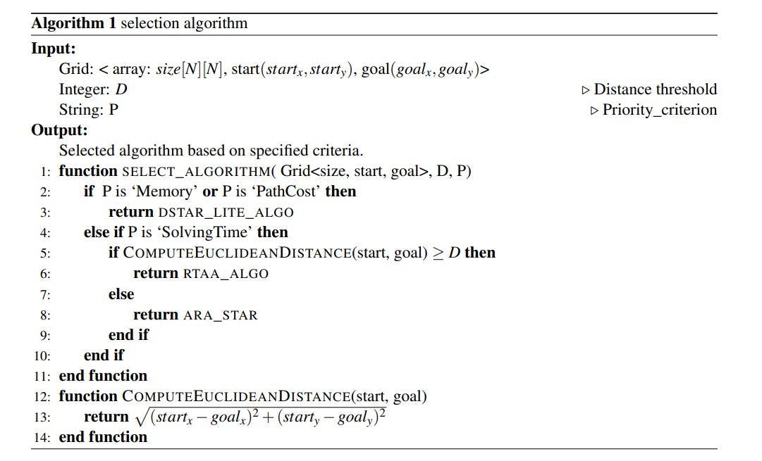
Based on the insights derived from our experimental results, we propose the selection algorithm represented in Algorithm 1. The algorithm is designed to select the appropriate search algorithm based on various priorities alongside the characterization of the environment used.

The selection algorithm emphasizes the desired priority first, which could manifest in various aspects of pathfinding tasks, including the path cost, memory usage, or the time taken to find a solution. The rational reason for emphasizing ”Priority” at the beginning of the selection algorithm is that, based on this user choice, different search algorithms may be considered to suit best the addressed problem. Thus, by tackling the ”Priority” upfront, The selected algorithm will eventually, cater to the main requirements of the task at hand.

The algorithm takes as input the Grid that is of size NxN with the start and goal positions, the distance threshold, and the priority criterion. If we aim to minimize memory usage, path cost, or both (Line 2), the algorithm suggests using D* Lite. However, If minimizing the solving time is our primary concern (line 4), we should first calculate the Euclidean distance between the start and the goal using the function in line 12. If the distance is higher or equal to the threshold (in our experiments it is equal to 140), the algorithms suggest using RTAA*. If the distance is less, then the selection algorithm suggests using ARA*.

5.1 Example of execution

To showcase the efficiency of our selection algorithm, we have designed an execution example that consists of generating a grid with random parameters i.e., choose a random grid size, obstacle density, and start to goal distance. After that, we generate an identical grid, however, we change only one parameter each time while keeping the other parameters as they were in the initial grid. We do the same for generating personalized grid environments, where we generate a grid with a random choice of wall number, and then we change the wall lengths.

We run RTAA*, ARA*, and D*Lite algorithms on the generated grids (all obtained results are shown in table 1) alongside our selection algorithm, so that we can compare the obtained results with what the selection algorithm is suggesting to use for the given grid.

It is essential to highlight that the randomly chosen values for the grid parameters are all within the range of the values used in the experiments, which ensures that the thresholds chosen are relevant. Also, the reason behind using only RTAA*, ARA*, and D*Lite in this execution example is because of their standout performance in our experiments.

For each grid, we run our selection algorithm each time with a different priority, and it suggests using an algorithm that will perform the best given the selected priority. The highlighted values in the table refer to the outcomes derived from the suggested search algorithm by our selection algorithm. These highlighted values are notably the best that we can obtain for each grid given a certain priority except for the red one; yellow represents the most efficient paths, green represents the best values that we can obtain if we want to reduce memory consumption, and the values highlighted in purple indicates the best solving time. However, our algorithm failed in selecting the right algorithm to use in the fourth grid when prioritizing the solving time, where the shortest solving time was found by RTAA*, instead our algorithm suggested using ARA*.