Examples of Merkle Tree Restructuring Algorithm—Execution and Example 1: Restructuring a Binary
by byRestructure Technologies@restructure
Technology is forever restructurable. The future belongs to whoever restructures it.
September 10th, 2024


Technology is forever restructurable. The future belongs to whoever restructures it.
Story's Credibility


Technology is forever restructurable. The future belongs to whoever restructures it.
Story's Credibility
About Author

Technology is forever restructurable. The future belongs to whoever restructures it.
Comments