


May 01, 2017
49,462 reads
Unveiling the Power of PM and P3M Algorithms on GPUs
by Aleksei OzeritskiiNovember 15th, 2023
Too Long; Didn't Read
TL;DR: This article explores the implementation and performance of the PM (Particle Mesh) and P3M (Particle-Particle Particle-Mesh) algorithms on GPUs, highlighting their efficiency in astrophysical simulations. Using GLSL language and Vulkan API, the algorithms are adapted for compatibility with a wide range of GPUs, including mid-range gaming graphics cards and integrated GPUs like Apple's M1 and M2.In the quest to simulate cosmic expanses and the intricate dance of celestial bodies, algorithms such as Particle-Mesh (PM) and its more nuanced counterpart, Particle-Particle-Particle-Mesh (P3M), have revolutionized our computational approach. These methods, which are deeply rooted in the seminal work of Hockney and Eastwood, provide a powerful framework for simulations, which I've explored and implemented with the help of modern GPU capabilities.
Based on my peer-reviewed paper "
PM and P3M Algorithms: A Primer
The PM algorithm works by assigning masses to a regular grid, solving the Poisson equation for the potential, and then differentiating the potential to obtain forces. This method simplifies the n-body problem, making it computationally feasible.
The P3M algorithm extends PM by incorporating short-range corrections via direct particle-particle interactions, resulting in improved accuracy in force computations without significantly increasing computational load.
GPU Implementation: A Leap in Performance
Going into greater detail, my implementation of the PM algorithm makes use of the versatility and power of the GLSL language and Vulkan API, ensuring compatibility across a wide range of graphics cards, from integrated Intel GPUs to the robust Apple M1 chips. Here is how I customized the PM algorithm for the GPU:
First Stage: Point Partitioning
The first stage involves partitioning points within parallelepipeds, laying the groundwork for the subsequent density assignment. We build 32x32 linked lists, each of which corresponds to a region in space. The goal is for each list to contain the indices of points in the corresponding parallelepiped.
We start by defining shared lists for each partition in GLSL using the compute shader:
// particles3_parts.comp - List Construction
const int nl = 32; // number of linked lists along one dimension
shared int lists[nl][nl];

// Initialize lists to -1
for (uint i = from; i < to; i++) {
    list[i] = -1;
}

lists[gl_LocalInvocationID.y][gl_LocalInvocationID.x] = -1;
barrier();

float h32 = l/32.0; // grid size divided by number of lists

// Build the linked lists by x, y coordinates
for (uint i = from; i < to; i++) {
    vec2 x = vec2(Position[i]) - vec2(origin);
    ivec2 index = clamp(ivec2(floor(x/h32)), 0, 31);

    // The head of the list for the area (index.y, index.x) is
    // in lists[index.y][index.x]
    // The previous list element is saved in list[i]
    // Each thread updates a unique element, so no synchronization is needed here
    list[i] = atomicExchange(lists[index.y][index.x], int(i));
}
...
After populating the shared lists, we have a structured overview of where each point lies within our space-partitioning grid. The GPU's atomic operations ensure that this process is both fast and accurate, laying the groundwork for efficient mass distribution in the PM algorithm's subsequent steps.
Take a look at this illustrative image to get a better idea of how these 2x2 linked lists are built and function within the larger context of our partitioning strategy:
This visualization depicts the process on a simplified 2x2 grid. In practice, a 32x32 grid is used, but the principles remain the same, albeit on a larger scale.
With our 32x32 linked lists ready, we move on to the mass distribution phase. We traverse the lists in a chessboard pattern here, which is not only systematic but also strategically designed to avoid race conditions when writing density values to our density array. This traversal is depicted in the following image, where the active lists being processed at any given time are highlighted in blue:
As we cycle through the particles in each list, we distribute their mass across the grid nodes. The chessboard-like processing pattern ensures that simultaneous writes to the density array from multiple threads do not interfere with each other, avoiding the classic problem of race conditions. This method improves the algorithm's efficiency while also ensuring data integrity.
The compute shader, which serves as the foundation of this initial setup, orchestrates the creation of linked lists within the GPU. For those who are interested in the actual code and its nuances, the compute shader responsible for this can be found on my GitHub repository:
Once our lists are established, we will traverse them in a chessboard pattern to avoid data races during mass distribution. The corresponding shader, which handles this traversal and density array construction meticulously, can also be viewed in detail here:
For the mass distribution, we use linear interpolation, leveraging barycentric coordinates to weigh the mass across the grid nodes. This technique ensures a smooth and continuous mass transition, which is critical for simulating physical systems. Consider the image below, which depicts the mass distribution using the Cloud-in-Cell (CIC) method:
The use of linear interpolation for mass distribution is a technique that mirrors physical reality by ensuring that the influence of a particle is felt across its immediate vicinity in a manner proportional to its position within a cell.
Poisson's Equation and Fast Fourier Transform
Solving Poisson's equation to calculate gravitational potential from mass distribution is a critical component of the PM algorithm. In my implementation, I use variable separation and a Fast Discrete Real Fourier Transform (FDRFT), adapting the algorithm described in A. A. Samarskii and E. S. Nikolaev's book "Numerical Methods for Grid Equations." This adaptation was specifically designed for GPU execution, leveraging its parallel processing capabilities to improve computational performance.
The shader code responsible for this part of the computation is complex, reflecting both the complexities of the mathematical procedure and the optimizations required for GPU use. The shader is proof of modern computing platforms' power and ability to handle calculations that were previously the exclusive domain of supercomputers.
For a more in-depth look at this process, please see the shader that handles the Poisson's equation using FDRFT on the GPU:
The P3M Algorithm and GPU Acceleration
The P3M (Particle-Particle Particle-Mesh) algorithm improves on the PM (Particle-Mesh) algorithm, particularly in how it computes local forces using Newtonian mechanics. While both algorithms share common ground, the P3M algorithm adds an extra layer of precision by partitioning points into cubes rather than parallelepipeds, improving the granularity of the mass distribution and force computation.
Advancing to Cubic Partitioning
The P3M implementation involves additional partitioning using lists, which is similar to the PM algorithm but takes a step further to accommodate cubic volumes. This additional step, which closely follows the classic Newtonian formulation, allows for a more precise calculation of local forces.
Computing Newtonian Forces in Parallel
The calculation of these local forces in parallel employs a classic parallel algorithm, which is finely detailed in the paper "
The shader codes that power these computations can be examined in greater depth by visiting the following links:
- For the sorting process that prepares the data for force calculations:
particles3_pp_sort.comp shader . - For the parallel force computation itself:
particles3_pp.comp shader .
Final Steps with Vertex Shader
The calculation of velocities and positions is the culmination of the P3M algorithm on the GPU. This is accomplished deftly with the Velocity Verlet algorithm, an integration method that provides a symplectic solution—ideal for conserving energy over long simulations, which is critical for accurate astrophysical results. The shader responsible for these final calculations can be found here:
The Velocity Verlet algorithm is a pillar of computational physics, providing stable and efficient computations of particle trajectories. For those who are unfamiliar with the Velocity Verlet algorithm, a primer can be found on its
Performance Benchmarks
Our implementations have resulted in significant performance improvements. The following table summarizes the benchmarks:
|
Stage |
M1 (CPU) |
M1 (GPU) |
Nvidia 3060 |
|---|---|---|---|
|
Density |
9.45 |
11.61 |
2.26 |
|
Potential |
8.87 |
5.69 |
0.86 |
|
Force |
313.93 |
103.09 |
28.87 |
|
Positions |
82.74 |
8.38 |
33.54 |
In the performance comparison table, we look at the execution time of each stage of the algorithm, measured in milliseconds across different processors: Apple M1 (CPU), Apple M2 (GPU), and Nvidia 3060. For the CPU version of the algorithm, OpenMP was utilized. The data from this table reveals a significant performance difference: the algorithm on the Nvidia 3060 runs 13 times faster compared to its execution on the Apple M1 CPU. These calculations were conducted with one million particles and a grid size of 64x64x64.
The P3M Algorithm and GPU Acceleration: A Note on Performance
When it comes to GPU acceleration, the P3M and PM algorithms present some computational challenges. Atomic operations and the management of linked lists, in particular, are not inherently optimal for GPU architectures. Despite this, the bottlenecks of these algorithms are located elsewhere.
Bottlenecks in Performance
The primary bottleneck in the PM algorithm is updating the density matrix, which requires significant memory bandwidth and synchronization between GPU threads. This limitation is vividly highlighted in a performance analysis using NVIDIA Nsight Graphics, as shown in this screenshot:
The P3M algorithm, on the other hand, has a bottleneck in the computation of local forces, which requires intensive floating-point operations and data shuffling between GPU threads and memory. This performance barrier is also visible in a detailed Nsight Graphics analysis, as shown in this screenshot:
Future Optimizations
Recognizing these performance bottlenecks, the program's next iterations will concentrate on addressing these issues. The efficiency of these calculations is hoped to be significantly improved through careful optimization and possibly leveraging new GPU features or architecture improvements.
While these challenges are not trivial, the solutions will not only improve the performance of the P3M and PM algorithms but may also contribute to the broader field of computational physics, where such algorithms are widely used.
Further Insights
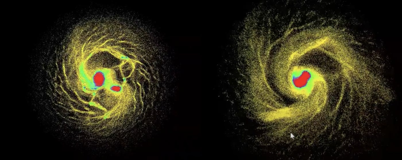
For those interested in learning more about these simulations, check out these YouTube videos that show the calculation of a galaxy's evolution and the dynamics of the early universe:
In the simulation video linked above, the Friedman universe model has been used to account for the expansion of the universe. This model describes a universe filled with homogeneously distributed fluid with pressure and energy, which governs the observed dynamics of cosmic expansion. For a more in-depth understanding of this model, see the
Finally, for enthusiasts and fellow developers, the source code for these algorithms, written in GLSL and using the Vulkan API to ensure compatibility across various GPUs, including Intel integrated graphics and Apple's M1, is available on GitHub:
Conclusion
In conclusion, modern mid-range gaming graphics cards and integrated GPUs are proving to be quite capable of accelerating numerical computations. The algorithms presented are implemented efficiently, with GPU computation times comparable to cluster processing across multiple nodes. The findings are consistent with those of other researchers, confirming the accuracy of this approach. The developed program can serve as a solid foundation for particle-based computational physics problems. Subroutines like the one for solving Poisson's equation could be applied to more complex hydrodynamic problems.
One key advantage of the approach described here is the ability to use a personal computer for rapid, parameter-varying numerical experiments with the luxury of real-time observation of evolving changes without the need for intermediate file storage or separate visualization software. While not all aspects of the algorithm perform optimally on GPUs (for example, mass distribution on the grid), careful optimization of GPU parameters such as computation partitioning, stream counts, and shared memory usage within thread groups has the potential for significant performance gains.
L O A D I N G
. . . comments & more!
. . . comments & more!